0 Intr oduction

In the context of the transition to decarbonization, one of the most effective ways to provide electricity consumers is the use of autonomous power supply systems[1-3]. Earlier, in [4-12], clarifications were proposed to the classification of autonomous power supply systems (APS), in particular, APS with a capacity of up to 10 kW and over 10-100 kW were introduced and justifications for these proposals were given.

If in APS with a capacity of up to 10 kW it is recommended to make the power supply scheme with two-wire lines with wires insulated from the ground, sinc e in such systems single-phase electric receivers will be used as consumers of electric energy [13-18], then in APS with a capacity of up to 100 kW the presence of three-phase consumers is possible.

The scope of application of APS with a capacity of 10-100 kW is currently extensive.They can be used in the following cases:

in the absence of cen tralized power supply;

if it is not possible to connect to the centralized power supply system;

remote object s;

dachas, small houses, trade stalls;

remote warehouses, cabins, houses at recreation centers;

for power, remote video surveillance and communicati on;

for power supply of fire and security alarms;

weather stations;

auto coffee shops;

autotourism, etc.

Basically, such systems are used to provide electricity to private households, farm s, such as apiaries, cheese dairies and greenhouses [19-21]. As a power source, photovoltaic(solar) batteries and wind turbines are in the most popular demand. It is economically inexped ient to provide for the presence of an energy service in the structure of such enterprises.

When switching to autonomous power supply systems,a number of issues should be solved,one of which is uninterrupted [22]. Because one problem that remains to this day is either low efficiency or the inconsistency of the primary source (wind, water, etc.).

In this direction, many methods and technical solutions have been applied and found their application [14-17].However, all the proposed technical solutions can be effectively implemented only if the actual loads[18-21] and the predicted electricity consumption are known. In the direction of forecasting electricity consumption, in particular for autonomous power supply systems, many methods have also been proposed, and in recent years, the use of neural networks and artificial intelligence has increased the accuracy of forecasting.

However, during the operation of these systems, a problem arises related to establishing the causes of constant failures, reliability and energy efficiency associated with frequent untimely failure of equipment, sources of autonomous power supply systems. The problem of compliance of the actual specific power of the electric load with the specific power in apartment buildings [1-7] and individual residential buildings [8] has become significant in recent years.

The term ‘‘actual specific power of the electric load” is understood as the ratio of the average monthly (obtained from the data of electricity meters installed at consumers of apartment buildings) or at peak hours (based on the results of measurements at morning and evening peaks at the entrance to apartments) to the number of days and hours in the month or at peak hours.

Whereas the term ‘‘specific power of the electric load” is understood as the ratio of the design capacity to the number of apartments, taking into account the presence or absence of gas supply and centralized hot and cold water supply at consumers (apartments).

Their inconsistencies, noted in works [1-7,9], lead already at the design stage of the power supply system of apartment buildings and individual residential buildings to the creation of preconditions for disruption of the operating mode of the elements of the 6-10/0.4 kV electrical distribution network.Numerous studies conducted by various groups of scientists for the Republic of Tatarstan, a number of cities of the Russian Federation (Moscow,Moscow region)[26] and the Chelyabinsk region[27] show that the specific power exceeds the actual specific power of the electrical load, while at the same time there are practically no similar studies for individual residential buildings.

As is known, the most accurate way to establish the correspondence between the actual specific power of the electric load and the specific power is to carry out measurements (30 min, hourly), which allows us to determine the actual specific power of the electric load of the apartment in the AB at the current moment. However,due to the increase in the actual specific power of the electric load, associated with a number of factors[26], the use of the results obtained on the basis of electric load measurements for predicting electricity consumption is not always correct, difficult and expensive. The costs are due,first of all,to the need to carry out repeated measurements with a frequency of 2-3 years.To adjust the specific power.

The most appropriate way to determine the actual specific power of the electric load is to use the average monthly electricity consumption data. It should be noted that using the results of previous electricity consumption to predict the electric load without identifying the factors that form the expected electric load of apartments leads to large errors and, as a result, requires adjustment based on measurements.

Therefore, in order to minimize the cost of money and time, as well as to eliminate the constant adjustment (every 2-3 years) of specific power in current realities, it is possible to predict the expected actual specific power of the electrical load of apartments in apartment buildings and individual housing buildings based on data on average monthly electricity consumpt ion, while taking into account the factors that create these loads.The article consists of the following chapters: Materials and methods of research.Comparison of results and their analysis.Simulation results. Discussion of results and conclusions.Conclusion.

1 Materials and research methodology

On the basis of previous studies, factors were i dentified[23-26], the generalization of which made it possible to propose an A coefficient that takes into account household consumers who receive power from both combined sources(traditional (T)) and single sources (for example, completely from renewable energy sources - hydraulic, solar,wind, etc.), (E) [26].

where tiis the temperature coefficient (taking into account the territorial-meteorological factor);

his a coefficient that takes into account the location of consumers above sea level;

cis the coefficient that takes into account the structural design of the residential building;

sis the coefficient of material (financial) well-being of the consumer (consumer welfare is an analogue of the income of the To¨rnqvist function, taken in the range from 0 to 1). The growth of this coefficient indicates the consumer’s ability to use the maximum number of household electric receivers;

kis a coefficient that takes into account the dynamics of the consumer’s welfare (a different number of electric receivers for abnormal electricity consumers). The temperature coefficient ti isdetermined depending on the ambient temperature at the consumer’s location:

The denominators of Eqs.(1) and(2)allow us to establish the influence of other energy sources (except electrica l)on electricity consumption and electrical loads.

Justification of the coefficients given in Eqs.(1) and (2).

The temperature coefficient t i is determined depending on the ambient temperature at the consumer’s location:

where: tmm tmean monthly temperature, ⁰C;

tt d b s l cthe difference between the temperature measured at sea level and at the consumer, ⁰C;

tm a a t s lmonthly average ambient temperature sea level, ⁰ C;

ta ma taverage monthly additional temperature ((the difference between the optimal and permissible temperature in the apartment) according to State Standard 30494-2011), ⁰C.

The coefficient for taking into account the difference in altitude above sea level is determined h x y :

The main equations of the mesoscale atmospheric model TSUNM3 are obtained for the Reynolds-averaged differential equations of hydrothermodynamics [28,29] in a coordinate system associated with the Earth’s surface,under the following assumptions [30]:

1) Mesoscale density variations are quasi-stationary.

2) Molecular diffusion is assumed to be negligible with respect to turbulent exchange.

3) Phase transitions of moisture, short-wave and longwave radiative heat exchange with explicit repres entation in the atmosphere are taken into account.

The mathematical model TSUNM3 includes the following equations:

Continuity equation [34]

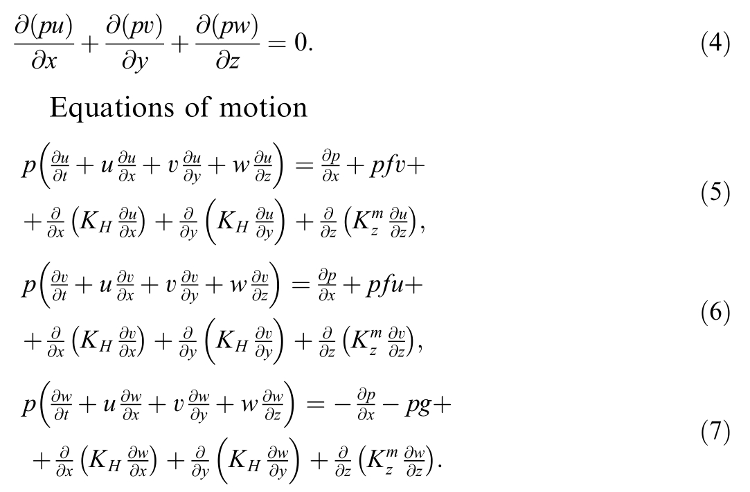
Here t-time; u, v, w-longitudinal, transverse and vertical components of the averaged wind speed vector in the direction of Cartesian coordinates x, y, z; pdensity;f Coriolis parameter; KHhorizontal diffusion coeffi-cient; coefficient of vertical diffusion of momentum;g acceleration of gravity; ppressure.Energy balance e quation

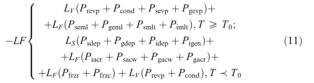
Here T absolute temperature; θvirtual potential temperature;CPheat capacity of air at constant pressur e;p0 101300H m2 R0 gas constant; Qradheating (cooling) of the atmosphere due to radiative long-wave and short-wave heat flows propagating in the humid atmosphere; p L Fchange in temperature due to phase transitions of moisture in the atmosphere; coefficient of vertical diffusion of heat and moisture; qvspecific density of water vapor in the atmosphere.

Equation of state

To model the processes of phase transformations of water moisture in the atmosphere, this paper uses the 6-class scheme of moisture microphysics WSM6 [31], developed by Korean scientists Hong and Lim for the wellknown mesoscale meteorological model WRF[32]. It considers six states of atmospheric moisture (water vapor,cloud moisture, rain moisture, ice particles, snow, graupel(hail)). For each of the parameters of the state of moisture in the atmosphere, a transfer equation is used, which,along with advective transfer, includes various parameterizations of physical processes leading to a change in the phase state of the considered forms of moisture state.The main equations of the WSM6 scheme are as follows:

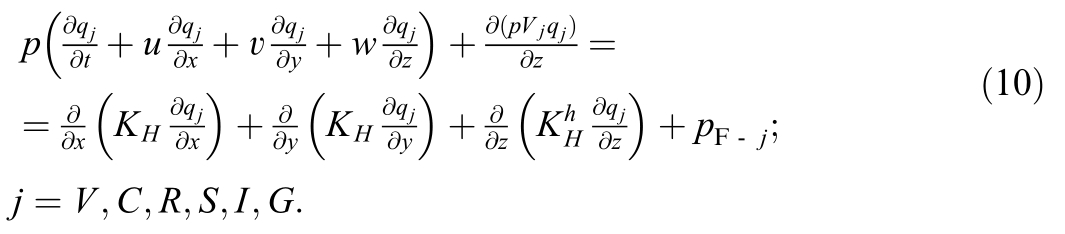
Here qV q C q R q S q I qG mass concentrations of water vapor, cloud moisture, rain moisture, snow, ice crystals and cereals in the atmosphere; V jsettling velocity of the j-th component [31].

In Fig. Fig. 1 shows a diagram of the microphysical processes of moisture in the WSM6 scheme [31].

The source terms of the equations Φj for the j-th class represent a mathematical notation of the parameterization of the transitions of atmospheric moisture from one state to another in accordance with Fig. 1 [33]. Some of the transitions occur at positive air temperatures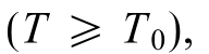and some at negative tempe ratures

The change in temperature due to phase transitions of moisture in the atmosphere in(8) is represented as follows:

The considered parameterization of atmospheric moisture microphysics has proven itself to be quite effective in forecasting precipitation [34].

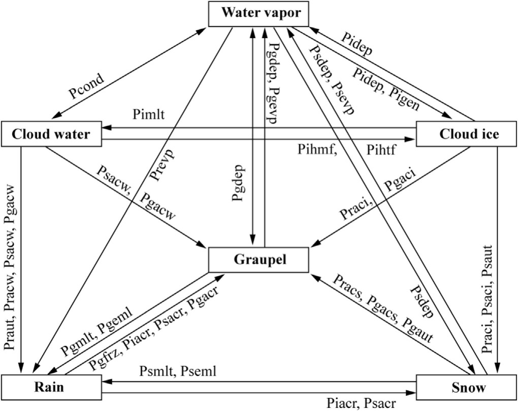
Fig. 1. Diagram of microphysical processes of moisture in the WSM6 scheme (taken from the article [22]).

For the system of Eqs. (4)-(10), before its numerical solution by the grid method, a coordinate transformation of the form [28] was app lied:

Here H height of the study area; h xythe height of

Transformation (12) allows mapping a threedimensional region with a curved lower boundary onto a parallelepiped.

Note, however, that as a result of performing su ch a transformation in (4)-(10), mixed derivatives appear in the new variables. Indeed, the differential equatio ns from the formulation (4)-(10) can be written in the following form [35]:the underlying surfa ce relief above sea level.

where Fa generalized scalar quantity that can represent any component of velocity, virtual potential temperature,specific humidity; Gdiffusion coe fficient of the quantity F.

Coefficient of structural design of buil dings and premises:

where: toptoptimal temperature in apartments, ⁰C.

k is a coefficient that takes into account the dynamics of consumer welfare (different numbers of electrical receivers among abnormal consumers of electricity).

where: Pactual specific poweractual specific power, kW.

W average monthlyaverage monthly electricity consumption, kWh; nd number of days in a month; Tday number of hours in a month; Pspeci fic rated powerstandardized specific power, kW [23-25].

The developed generalized coefficient Ai in combination with the data of the average monthly electricity consumption make it possible to determine the average daily electric load of apartments in apartment buildings and private housing construction. Next, let’s present the formula for the average daily calculation of electric power taking into account the generalized coefficientAiT :

where: Ai Tis the generalized coefficient.

To determine the electrical load during maximum hours, taking into account the proposed generalized coefficient AiEand the maxi mum load time coefficient under conditions with a single energy source [23], it is proposed to use the following equation:

where: αml tis the maximum load time coefficient.

As is known, the hours of maximum load are observed in the winter period (the so-called morning and evening maximum). To derive a coefficient characterizing the maximum consumption of electricity based on long-term observations, the estimated time of maximum load was taken for Dushanbe as 6 h (with an altitude of 767 m above sea level), and for the cities of the Gorno-Badakhshan Autonomous Region, Khorog (with an altitude of 2200 m above sea level) 7 h per day [24].

2 Simulation results

Using the data on average monthly electricity consumption for 226 apartments in apartment buildings (obtained from the readings of electricity meters installed in apartments of apartment buildings)Figs. 2 and 7 individual residential buildings Fig. 3 for 2022, obtained from the energy supply organization of the city of Chelyabinsk and with different territorial and meteorological factors of cities (location of apartment buildings above sea level and climatic factors) of the Republic of Tajikista n, the average daily actual power electrical loads of apartments in apartment buildings for the same month as for the city of Chelyabinsk were calculated in January (see Figs. 4 an d 5).

Using the example of one apartment, we will present the sequence of calculating the average daily electric load taking into account the generalized coefficient of Ai(T)for the city of Chelyabinsk.

1) Determination of the temperature coefficient ti. For this purpose, the average daily temperature of the object of study (apartment) - tm.m.t for January 2022 and the average daily temperature at sea level- tm.a.a.t.s.l were obtained from the archive data(Internet world-weather.ru). The results are presented in the form of Fig. 6 for the city of Chelyabinsk and Fig. 7 for the cities of Dushanbe and Khorog of the Republic of Tajikistan (RT).

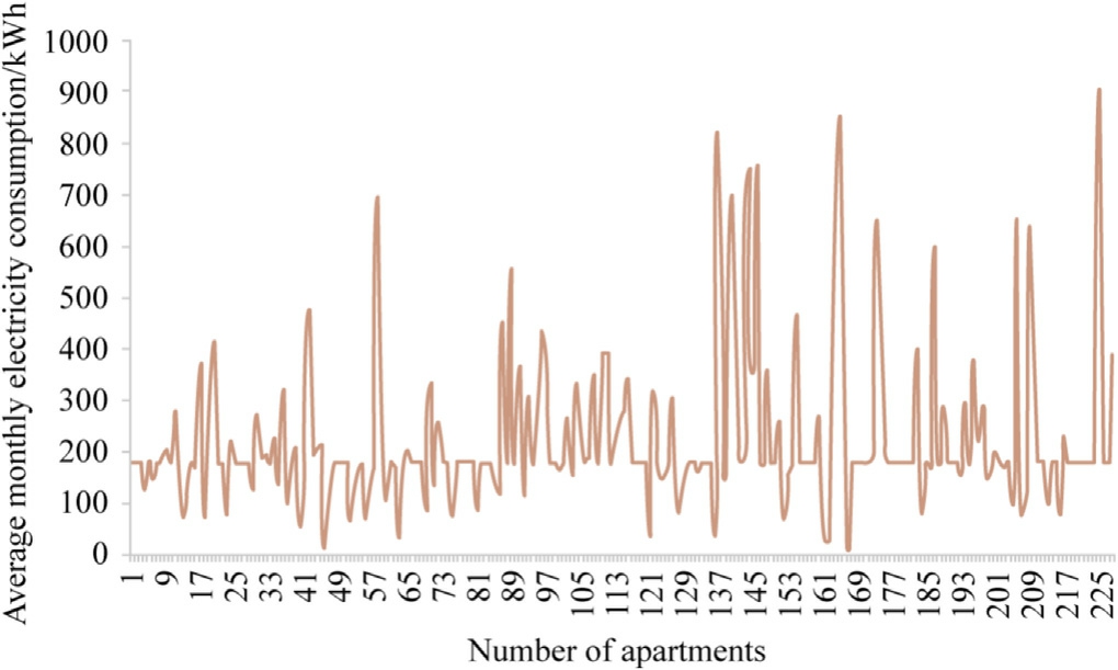
Fig. 2. Average monthly electricity consumption for 226 apartments in an apartment building, averaged per apartment (on electric stoves and with centralized hot and cold water supply).

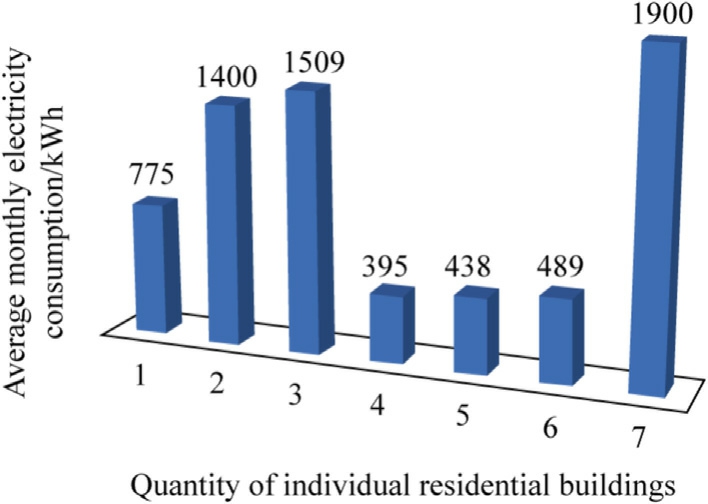
Fig. 3. Average monthly electricity consumption of individual residential buildings.

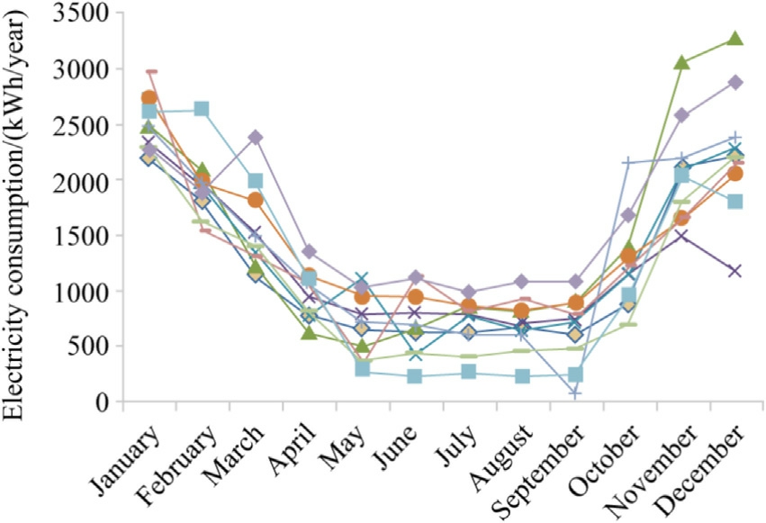
Fig. 4. Average monthly electricity consumption by apartments in multiapartment buildings, averaged per apartment in the city of Dushan be(located at 767 m above sea level without gas supply and centralized hot and cold water supply).

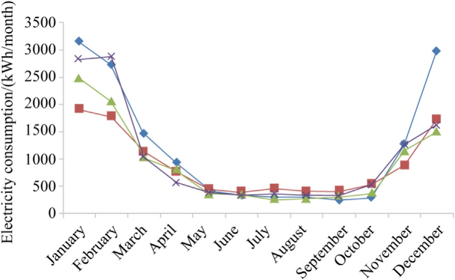
Fig. 5. Average monthly electricity consumption by apartments in multiapartment buildings, averaged per apartment in the city of Khorog(located at 2200 m above sea level without gas supply and centralized hot and cold water supply).

Substituting the results given in Fig. 6 in (3), determine the temperature coefficient ti for the 1st day of January 2022 of one apartment.

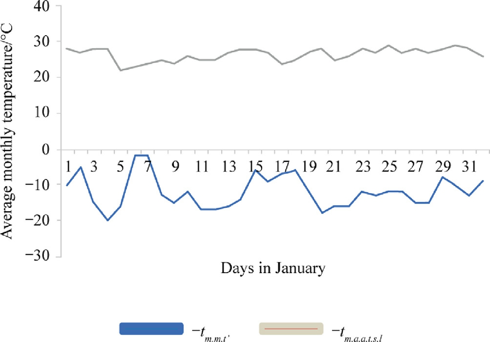
Fig. 6. Average daily temperature of the research object (apartment).

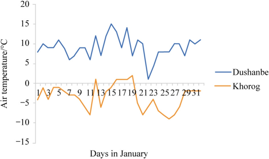
Fig. 7. Average daily air temperature of the research objects (apartments)located in the cities of Dushanbe and Khorog.

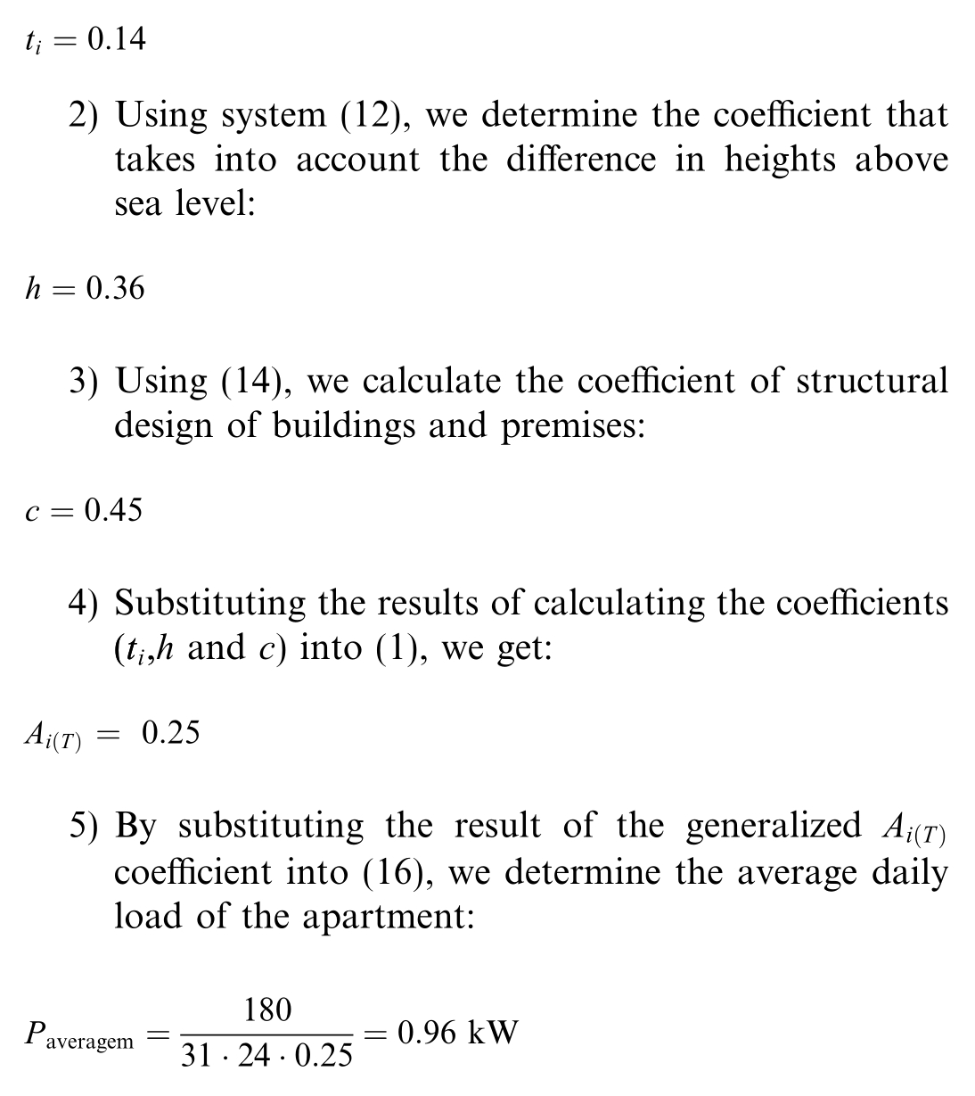
Similarly, for other days (January 2022), a generalized coefficient of Ai(T) was calcul ated. The results are presented in the form of Fig. 8 for Chel yabinsk.

Based on the data on average monthly electrici ty consumption presented in Figs. 2 and 3 for the city of Chelyabinsk and the values of the generalized coefficient (1) (see Fig. 8), we determine the values of the change in the actual specific power of the electric load by day (January 2022)for apartments in multi-apartment buildings Fig. 9 and for individual housing buildings Fig. 10.

Whereas according to the data on average monthly electricity consumption presented in Figs. 4 and 5 for the cities of Dushanbe and Khorog, using the generalized coefficient(2) taking into account territorial and meteorological factors (see Fig. 7), we determine the values of the change in the actual specific power of the electric load by day (January 2022) for apartments in multi-apartment buildings and for the city of Dushanbe Fig. 11 and the city of Khorog Fig. 12 of the Republic of Tajikistan.

As can be seen from the above results of calculating the average daily actual specific power of the electric load,Figs. 8-11, the value of the actual power is lower than the data given in the set of rules. However, the value of the actual specific power of the cities of Dushanbe and Khorog in relation to the city of Chelyabinsk is 2 times higher. This once again confirms that the absence of other energy sources is the reason for the increase in electricity consumption due to the increase in the number of connected electrical receivers in households [26]. Next, using(17), according to the average monthl y electricity consumption data (see Figs. 4 and 5), taking into account the obtained coefficient of the time of maximum load αmlt and the generalized coefficient Ai E ,changes in the electric load during peak hours by days of apartments in multi-apartmen t residential buildings were calculated with averaging per 1 apartment in Dushanbe and Khorog. The results are presented in Figs. 13 and 14.

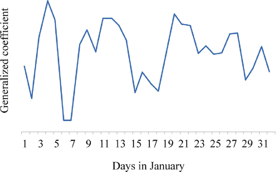
Fig. 8. Results of calculating the generalized coefficient for the city of Chelyabinsk.

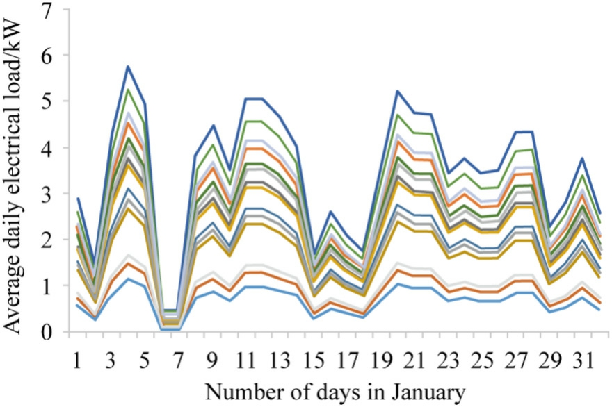
Fig. 9. Change in the actual specific power of the electrical load per day of apartmen ts in apartment buildings with averaging per 1 apartment in the city of Chelyabinsk.

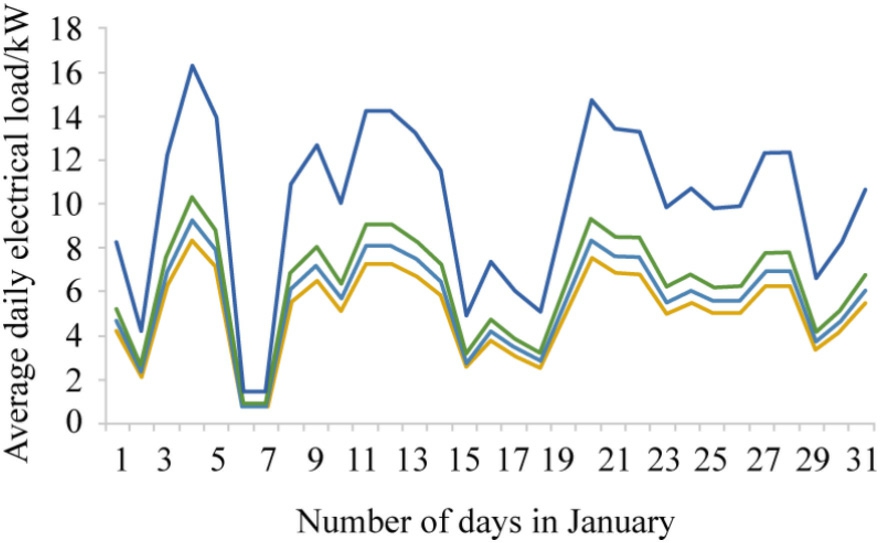
Fig. 10. Change in the actual specific power of the electrical load by day for an individual residential building, averaged per 1 apartment in Chelyabinsk.

As can be seen, the results of modeling the average daily actual specific power of the electric load for apartments in multi-apartment residential buildings and individual residential buildings based on the average monthly electricity consumption data taking into account the generalized coefficient (1) for the city of Chelyabinsk and the generalized coefficient (2) for the cities of the Republic of Tajikistan show that the actual power is low er than the installed specific power [26].

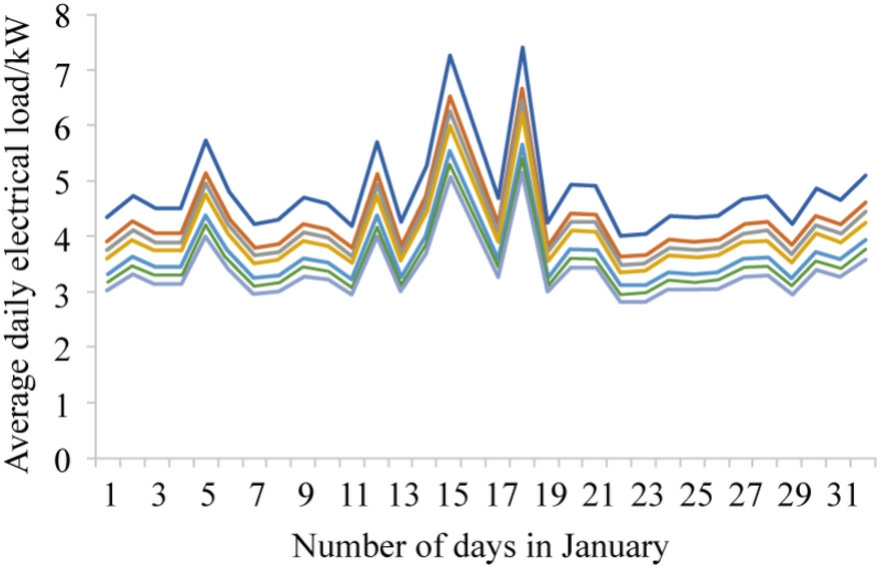
Fig. 11. Change in the actual specific power of the electrical load by day of apartments in apartment buildings with averaging per 1 apartment in Dushanb.

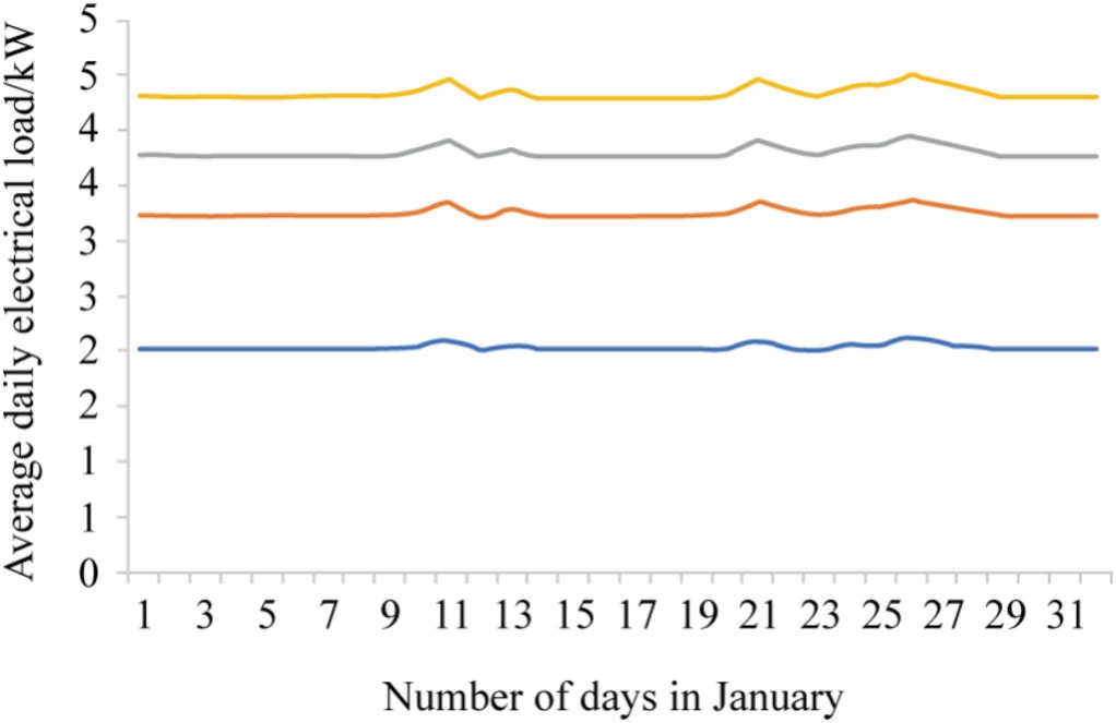
Fig. 12. Change in the actual specific power of the electrical load by day of apartments in apartment buildings with averaging per 1 apartment in the city of Khorog.

In turn, the modeling results showed high convergence with the results obtained earlier based on measurements for the city of Chelyabinsk [25]. However, due to the lack of other energy sources (gas supply and hot water supply)in the conditions of the Republic of Tajikistan and based on the obtained coefficient of the time of maximum load[23,25] and the generalized coefficient (2), the obtained values of the actual specific power exceed the maximum in hours by 1.2-2.5 times [26] the specific power specified by RB 256.1325800.2016 [27].

This, in turn, creates the preconditions for disruption of the operating mode of the elements of the 6-10/0.4 kV distribution electrical network, which will undoubtedly lead to a violation of not only the requirements of NP R 12.1.038-2024, but also the service life of the elements of the urban distribution electrical network.

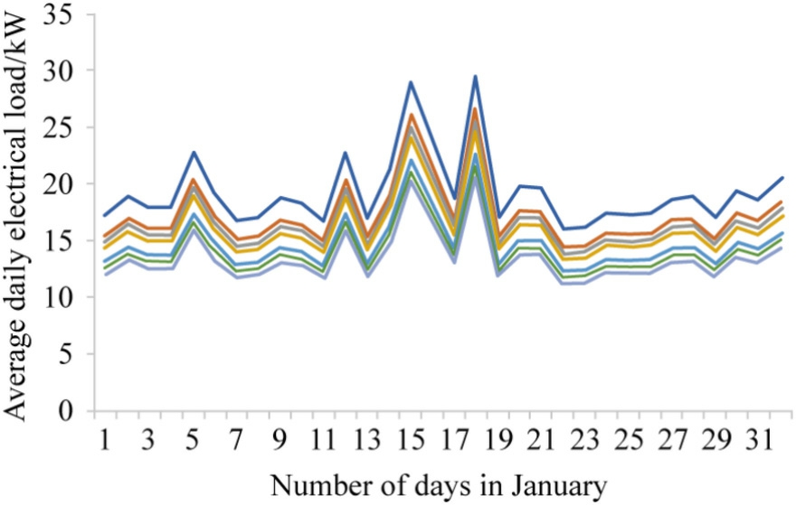
Fig. 13. Change in the actual specific power of the electrical load during peak hours by day in apartments in multi-apartment residential buildings with averaging per apartment in Dushanbe.

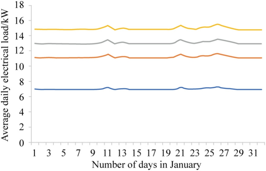
Fig. 14. Change in the actual specific power of the electrical load during peak hours by apartments in multi-apartment residential buildings with averaging per apartment in the city of Khorog.

3 Discussion of the resul ts and conclusions

The results of determining the actual specific electrical load based on the data of average monthly electricity consumption and the developed generalized coefficient Ai T ,obtained on the basis of the proposed model (16), showed that electricity consumers (apartments) in multi-apartment residential buildings and individual residential buildings for the city of Chelyabinsk and the cities of the Republic of Tajikistan unde r consideration have a power lower than those given in the rule book. Whereas during peak load hours in apartments of apartment buildings (17) of cities of the Republic of Tajikistan, the actual specific power is higher than those given in the set of rules. Thus, our proposed approach allows us to determine the actual specific power of the electrical load based on average monthly electricity consumption, taking into account the generalized coefficient A for apartment buildings and individual residential buildings with sufficient accuracy without carrying out a significant number of measurements.

Thus, by transforming the obtained (15) and (16) it is possible to identify the correspondence of the actual specific power consumption with the standardized specific power consumption due to the discrepancy between them.Thus, to increa se the accuracy of the forecast in power consumption and to increase the energy efficiency of power supply systems.

To check the adequacy of the proposed models, the results obtained were compared with the results of experimental data. For experimental data, the readings of electricity metering devices for groups of household consumers were taken. The comparison results are presented in Table 1.

The obtained results, presented in Table 1, show high convergence (errors do not exceed 5%). Thus, it can be stated that the forecast accuracy is high when using the proposed method (18). To compare the results obtained on the basis of(18) with the results of the selected and trained neural network model, the dependences of electricity consumption by household consumers for the considered number of cities for the period of 2022 were constructed, Figs. 15 and 16.

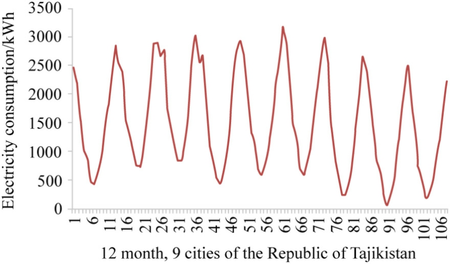
Fig. 15. Results of modeling by the proposed method.

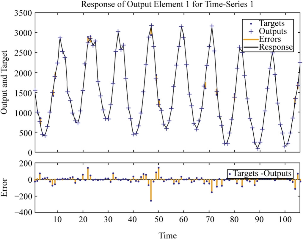
Fig. 16. Results of modeling in a neural netwo rk model.

Table 1 Comparison of experimental results with simulation results [26].

The obtained results, presented in Fig. 16, showed (as shown above) high convergence with the results obtained by the proposed method (18). Thus, having compared the results of the computer, neural network model, experimental data with the proposed methods, it can be stated about the high accuracy of forecasting electricity consumption when using the method.

4 Conc lusions

The proposed model based on the average monthly electricity consumption data and the developed generalized coefficient allows us to determine the compliance of the actual specific power with the specific power without longterm measurements. The results of the average daily actual specific electric load show that in apartment buildings and individual iron structures of the city of Chelyabinsk and cities of the Republic of Tajikistan, the actual specific power is lower than the standardized specific power, while during peak load hou rs in apartment buildings of the cities of the Republic of Tajikistan, the actual specific power is higher than those specified in the set of rules.

The substantiated and developed (1) and (2) and based on them (16-18) allow us to establish compliance of the actual specific power of the electric load with the standardized specific powers and, if there is a discrepancy, to reevaluate them. Thereby increasing the accuracy of the forecast of electrici ty consumption according to (18), which are confirmed by the results given in Table 1. This in turn will increase the energy efficiency of power supply systems, in particular in conditions where only renewable energy sources are used as a source. However, it is also necessary to note (2) has a limitation in application in conditions with critical meteorological conditions, since in these conditions,in the absence of other energy sources (gas supply and hot and cold water supply), a problem aris es with the high accuracy of determining the coefficient kand will require the use of additional means to limit them.

CRediT authorship contribution statement

Saidjon Tavarov: Supervision, Formal analysis, Writing- review & editing, Methodology, Conceptualization,Writing - original draft. Aleksandr Sidorov:. Andrey Svyatykh:. Yulia Medvedeva:. Olga Khanzhina:.

Declaration of competing interest

We declare that we have no conflict of interest.

References

[1]K.V. Blazakis, T.N. Kapetanakis, G.S. Stavrakakis, Effective electricity theft detection in power distribution grids using an adaptive neuro fuzzy inference system, Energies 13 (12) (2020)3110.

[2]F. Issi, O. Kaplan, The determination of load profiles and power consumptions of home appliances, Energies 11 (3) (2018) 607.

[3]F. Ziel, Load nowcasting: predicting actuals with limited data,Energies 13 (6) (2020) 1443.

[4]L. Foltyn, J. Vysocky´, G. Prettico, et al., OPF solution for a real Czech urban meshed distribution network using a genetic algorithm, Sustainable Energy Grids Networks 26 (2021) 100437.

[5]A. Ahmad, N. Javaid, A. Mateen, et al., Short-term load forecasting in smart grids: an intelligent modular approach,Energies 12 (1) (2019) 164.

[6]R. Ahmed, V. Sreeram, Y. Mishra, et al.,A review and evaluation of the state-of-the-art in PV solar power forecasting: techniques and optimization, Renew. Sustain. Energy Rev.124(2020)109792.

[7]G. Angelini, L. De Angelis, Efficiency of online football betting markets, Int. J. Forecast. 35 (2) (2019) 712-721.

[8]D. Apiletti, E. Pastor, Correlating espresso quality with coffeemachine parameters by means of association rule mining,Electronics 9 (1) (2020) 712-721.

[9]J. Barker, Machine learning in M4: what makes a good unstructured model?, Int. J. Forecast. 36 (1) (2020) 150-155(LinkOut).

[10]J. Boylan, A. Syntetos, Intermittent Demand Forecasting -Context, Methods and Applications, Wiley, 2021.

[11]J.W. Burton, M.K. Stein, T.B. Jensen, A systematic review of algorithm aversion in augmented decision making,J.Behav.Decis.Mak. 33 (2) (2020) 220-239.

[12]F. Chan, L.L. Pauwels, Some theoretical results on forecast combinations, Int. J. Forecast. 34 (1) (2018) 64-74.

[13]A. Choudhury, E. Urena, Forecasting hourly emergency department arrival using time series analysis, Br. J. Healthc.Manag. 26 (1) (2020) 34-43.

[14]F.X. Diebold, M. Shin, Machine learning for regularized survey forecast combination: partially-egalitarian LASSO and its derivatives, Int. J. Forecast. 35 (4) (2019) 1679-11169.

[15]N.N. Sergeev, P.V. Matrenin, Enhancing efficiency of ensemble machine learning models for short-term load forecasting through feature selection, in: Proceedings of 2022 IEEE 23rd International Conference of Young Professionals in Electron Devices and Materials (EDM), 2022 in Altai, Russian Federation, 2022, pp.368-371.

[16]Y. Fan, S. Nowaczyk, T. Roognvaldsson, Transfer learning for remaining useful life prediction based on consensus self-organizing models, Reliab. Eng. Syst. Saf. 203 (2020) 107098.

[17]C. Fezzi, L. Mosetti, Size matters: estimation sample length and electricity price forecasting accuracy, Energy J. 41 (4) (2020) 231-254.

[18]T.E. Goltsos, A.A. Syntetos, E. van der Laan, Forecasting for remanufacturing: the effects of serialization, J. Oper.Manag.65(5)(2019) 447-467.

[19]Y. Grushka-Cockayne, V.R.R. Jose, Combining prediction intervals in the M4 competition, Int. J. Forecast. 36 (1) (2020)178-185.

[20]H. Hewamalage, C. Bergmeir, K. Bandara, Recurrent neural networks for time series forecasting: current status and future directions, Int. J. Forecast. 37 (1) (2021) 388-427.

[21]T. Hong, P. Pinson, Energy forecasting in the big data world,Int.J.Forecast. 35 (4) (2019) 1387-1388.

[22]M. Senyuk, M. Safaraliev, A. Gulakhm adov,et al.,Application of the conditional optimization method for the synthesis of the law of emergency control of a synchrono us generator steam turbine operating in a complex-closed configuration power system,Mathematics 10 (21) (2022) 3979.

[23]S.S. Tavarov, A.I. Sidorov, O.O. Sultonov, Modell ing the operating mode of the urban electrical network and dev eloping a method for managing these modes, Math. Modell. Eng. Pr obl.8(5)(2021) 813-81 8.

[24]T.S. Shiralievich, S.A. Ivanovic, S.S. Mamanazarovna, et al.,Learning algorithm of artificial neural network factor forecasting power consumption of users, Bull. Electr. Eng. Inform. 11 (2)(2022) 602-612.

[25]A. Sidorov, S. Tavarov, Method for forecasting electric consumption for household users in the conditions of the republic of Tajikistan, Int. J. Sustain. Dev. Plan. 15 (4) (2020)569-574.

[26]S.S. Tavarov, I. Zicmane, S. Beryozkina, et al., Evaluation of the operating modes of the urban electric networks in Dushanbe City,Tajikistan, Inventions 7 (4) (2022) 107.

[27]Ministry of Construction and Housing of the Russian Federation(2016) Rule book 256.1325800.2016. Electrical installations of residential and public buildings.Rules of design and installation(in Russian). Standard Inform.

[28]V.V. Penenko, A.E. Aloyan, Models and Methods For Environmental Protection Tasks, Nauka, Novosibirsk, 1985.

[29]R. Pielke, Mesoscale Meteorological Modeling, Academic Press,San Diego, California, 2002.

[30]F.T.M. Niestadt, H. Van Dop, Atmospheric Turbulence and Modeling of Impurity Propagation, Gidrometeoizdat, Moscow,1985.

[31]S.Y. Hong, J.O.J. Lim, The WRF single-moment 6-class microphysics scheme (WSM6), J. Korean Meteorol. Soc. 42 (2)(2006) 129-151.

[32]J.G. Powers, J.B. Klemp, W.C. Skamarock, et al., The weather research and forecasting model: overview, system efforts, and future directions, Bull. Am. Meteorol. Soc. 98 (8) (2017) 1717-1737.

[33]J.W. Bao, S.A. Michelson, E.D. Grell, Pathways to the production of precipitating hydrometeors and tropical cyclone development,Mon. Weather Rev. 144 (6) (2016) 2395-2420.

[34]A.V. Starchenko, A.A. Bart, N.N. Bogoslovskiy, et al.,Mathematical modelling of atmospheric processes above an industrial centre, 20th Int. Symp. Atmos. Ocean Optics: Atmos.Phys. 9292 (2014) 929249.

[35]A.V. Starchenko, E.A. Danilkin, S.A. Prohanov,et al., Numerical prediction of local meteorological processes above a city with a supercomputer, J. Phys. Conf. Ser. 1740 (1) (2021) 012071.

Received 17 February 2025; re删vis除ed 26 March 2025; accepted 3 April 2025

Peer review under the responsibility of Global Energy Interconnection Group Co. Ltd.

* Corres删ponding au除thor.

E-mail addresses:tavarovss@susu.ru (S. Tavarov), sidorovai@susu.ru(A. Sidorov), svyatykh@mail.ru (A. Svyatykh), julyabakal@mail.ru(Y. Medvedeva), leka711@bk.ru (O. Khanzhin a).

https://doi.org/10.1016/j.gloei.2025.04.007

2096-5117/© 2026 Global Energy Interconnection Group Co. Ltd. Publishing services by Elsevier B.V. on behalf of KeAi Communications Co. Ltd.This is an open access article under the CC BY-NC-ND license(http://creativecommons.org/licenses/by-nc-nd/4.0/).

Saidjon Tavarov received PhD degree at South Ural State University (national research university), Russia, 2015. In 2008, he received a diploma of specialty in power supply of industrial enterprises from the Tajik Technical University, Dushanbe, Republic of Tajikistan,in 2023, he received a master’s degree in fire safety from the South Ural State University Russia. He is working in South Ural State University (national research university),Polytechnic Institute, and Associate Professor.The research area is aimed at improving the reliability of urban electrical networks.