0 Intr oduction

In many developing nations, the reliability of electricity supply remains constrained by a persistent mismatch between generation capacity and transmission infrastructure. This imbalance, compounded by rising demand, frequently leads to network overloading and large-scale blackouts, as seen in Pakistan, where significant portions of the trans mission system remain overloaded (NEPRA,2020). To address these grid challenges effectively, a granular understanding of residential consumption patterns through accurate household-level forecasting is essential.

Short-term electricity consumption forecasting plays a crucial role in demand-side management, energy optimization, and grid stability. Accurate predictions enable power companies and policymakers to anticipate peak demand,optimize energy distribution, and integrate renewable energy sources more effectively [1,2]. While much research has focused on forecasting at the regional or national level,although several studies have examined household-level forecasting, most rely on aggregated or simulated datasets.In contrast, real- time residential electricity consumption data is highly volatile, with minimal repeating patterns,making short-term forecasting particularly challenging.High-resolution household data from developing countries remains under-explored,despite its potential to enable personalized energy management. Consequently, demandside interventions at the household level have largely remained untapped [3-6]. Time series forecasting is a cornerstone of energy demand analysis, offering a robust framework for extracting meaningful patterns from historical consumption data to predict future trends. In the context of residential electricity consumption, where,residential electricity consumption data inherently exhibits temporal dependencies and seasonal fluctuations, time series models prove particularly valuable. Autoregressive Integrated Moving Average (ARIMA) models are adept at handling non-stationary time series, effectively capturing trends and irregular fluctuations often observed in electricity usage. However, residential consumption is rarely devoid of seasonal patterns, such as da ily peaks and weekly cycles influenced by lifestyle and weather variations.To address this,Seasonal ARIMA(SARIMA)models extend the capabilities of ARIMA by incorporating seasonal components.This allows for the explicit modeling of recurring patterns, such as daily and weekly consumption cycles, making SARIMA exceptionally well-suited for capturing the nuanced dynamics of household electricity usage[7]. Given the non-stationary and seasonal nature of residential electricity consumption, this study leverages both ARIMA and SARIMA models. By comparing their predictive performance, we aim to determine the most effective approach for short-term household-level forecasting, providing valuable insights for grid management and demand-side interventions.

To forecast residential electricity consumption, two broad modeling approaches exist: physical modeling,which relies on first principles to capture the underlying mechanisms of consumption [8,9],and style="font-weight: bold;">.

The rest of the paper is organized as follows: Section 2 reviews the literature on short-term electricity consumption forecasting, emphasizing recent advancements. Section 3 details the mathematical formulation, including time series modeling and clustering approaches. Section 4 presents the case study. Section 5 discusses insights from the clustering analysis; Section 6 discusses the case study with key findings and section 7 concludes potenti al directions for future research.

1 Literature revie w

This section reviews key literature on electricity consumption forecasting, highlighting various modeling techniques, the transition from aggregated to household-level analys is, and the integration of clustering methods to enhance prediction and policy relevance.

1.1 Aggregated consumption forecasting model

Most of the early work in electricity demand forecasting has focused on aggregated consumption, leveraging traditional time series models. An aggregated power consumption of twenty-three buildings has been used to build an ARIMA model in [5]. The authors also compared exponential smoothing models, ANN models, and NARX model, with the NARX achieving the lowest RMSE across all forecasting steps and lowest MAPE for most horizons(ranging from 1.87% at 1-step ahead to 6.16% at 24-step ahead). Similarly, in [17] the authors used aggregated power data and proposed ARIMA-based modeling as the most suitable model to forecast power consumption for a period of a day, a week or a month, with a reported MAPE of 5.994240. In [6], the authors applied ARIMA and ARMA models to aggregated consumption dataset from the Pakistan grid and found that ARIMA performed better for monthly and quarterly forecasting, achieving RMSE values of 0.09 for 6-10 month forecasts and 0.02 for the 2-quarter forecast. The proposed study employs household-level (non-aggregated) data to provide detailed insights into individual electricity consumption. This enables personalized demand- side management (DSM),improved control of appliances, and effective integration with building managem ent systems (BMS) for more effi-cient energy use. Although aggregated forecasts are useful for system-level planning, they cannot capture the variations at the household level. By focusing on nonaggregated data,the proposed study aims to optimize electricity use for individual consumers while also supporting overall grid stability.

1.2 Household-Level forecasting challenges and solutions

In the context of household electricity forecasting, Ma et al. [18] reviewed recent work specifically focused on family-level short-term electricity load forecasting, covering classical time series models (e.g., ARIMA), deep learning approaches (e.g., LSTM, CNN), and machine learning methods (e.g., SVR, Random Forests). However, they noted that deep learning methods may face issues like overfitting and instability, while machine learning techniques can struggle with non-linear and non-stationary data. In this paper we have also targeted the forecasting of individual houses’ power consumption. However, we have adopted time series-based modeling, and we have formulated both ARIMA and SARIMA based models for the prediction of power consumption and drew a comparison between their performances. Some attempts have also been made to forecast the consumption of individual buildings.These include a three-storey building power dataset used to forecast power consumption by the AR IMAX model(autoregressive integrated moving average with exogenous variables),where external variables such as outdoor temperature and occupancy-related login data were incorporated, where login data slightly improving model fit by reducing RMSE from 4.268 to 4.127 and MAPE from 1.244 to 1.21 [19]. Another study of fifteen houses’ consumption has also been conducted in[20] to predict future consumption using Support Vector Machine (SVM), with the model showing its best performance for Household 1,achieving a MAPE of 12.78 for daily prediction and 23.31 for hourly prediction. To further address household-level forecasting complexities, Mahmood et al. [9] introduced a hierarchical multi-resolution agent-based modeling(ABM) framework to simulate household electricity demand profiles, specifically modeli ng energy consumption patterns of multiple residential buildings.

As discussed earlier, the power system of Pakistan and other developing nations is underdeveloped. Most of the modeling exercises attempted in literature use aggregated power consumption data. Power consumption of individual houses has often been left out of scope due to the unavailability of consumption data. However, modeling individual houses is expected to be difficult because of limited periodicity in the consumption data. In this paper, we formulated consumption models for individual residential houses and we hope the modeling outcome could be beneficial for power managing authorities in decisionmaking and in the implementation of demand-side and supply strategies. The electricity consumption data is considered from individual houses in Lahore, Pakistan. The dataset is highly volatile in nature, and as noted, we used both ARIMA and SARIMA based time series modeling.For the simulation results, we have found that SARIMA models performed better on validation data. Their model orders are much lower in comparison to the ARIMA models and they have the capability to provide forecasts for longer periods in comparison to ARIMA models.

1.3 Advanced forecasting techniques and hybrid models

Several recent studies have explored hybrid and advanced techniques for improving forecasting performance. To analyze trends and limitations in forecasting techniques, Klyuev et al. [21] systematically reviewed electricity consumption forecasting methods across operational, short-term, medium- term, and long-term horizons, covering statistical models, machine learning techniques, deep learning methods, hybrid approaches,and fuzzy logic systems, highlighting key limitations in accuracy and adaptability and poi nting to the growing relevance of intelligent and hybrid solutions. Sari et al. [22]proposed a SARIMA-based method for forecasting electricity loads during major Indonesian religious holidays,such as Eid al-Fitr and Christmas Day, in East Kalimantan, using hourly load data from 2015 to 2018, where the best SARIMA (0,2,1)(0,1,0)24 model achieved a MAPE of 16.99% for Eid al-Fitr and 8.68% for Christmas Day.Similarly, in [23], Zhao used machine learning and time series analysis to forecast daily aggregated electricity consumption in Tetouan, Morocco, where a Random-Forestcorrected SARIMA model reduced the MAE from 944.903 to 562.767, thereby impr oving accuracy by about 40%. Similarly, the SARIMA model has also been used to predict electricity consumption in Yunnan Province by Yin et al [24] achieving a MAPE (mean absolute percentage error) of 6.05% using data from 2008 to 2018. Further optimizat ion and comparison of SARIMA with other models are presented in[25], with an emphasis on improving accuracy for both short- and long-term forecasts. In[26], a long short-term memory (LSTM) neural network was employed for gross electricity consumption forecasting in Tu¨rkiye, where it outperformed the SARIMA model and achieved a MAPE of 2.42%.Transitioning from recurrent to attention-based networks, Chan and Yeo [27] proposed a sparse transformer-based model for electricity load forecasting using historical consumption data,demonstrating competitive ac- curacy while being up to 5 faster during infer ence,although long time-series forecasting remains a broader challenge. Another advanced framework, B- SCN [28], was proposed for probabilistic short-term power load forecasting, where an adaptive boosting algorithm constructs an ensemble of SCN models to reduce random prediction and improve forecasting accuracy and stabili ty. The proposed model achieved an RMSE of 10.4%using half-hourly load data from an Australian region.Similarly,Zeng et al.[29] proposed a hybrid Prophet-BO-XGBoost framework for short-term load forecasting. They combined time-series trend modeling with nonlinear feature learning and further employed Bayesian optimization to fine-tune the hyperparameters of the XGBoost framework, enhancing accuracy and generalization in complex load scenarios, where the proposed model yielded an RMSE of 19.629 kW and a MAPE of 1.352% on regional load data from 2018 to 2020.

1.4 Clustering approaches for load profiling

Clustering of residential building load profiles has been investigated well to analyze occupants’ electricity consumption in order to assist demand-side management.Various cluste ring techniques have been published in the literature, e.g., k-means, fuzzy c-means, and hierarchical clustering methods to group different houses based on their power consumption. In [16], the authors introduced two techniques of clustering—hierarchical and selforganized map (SOM)—to identify groups of consumers responsible for high electricity consumption which eventually influences the utility peak. Electricity pattern recognition is investigated for large power consumers using different clustering methods in [30]. Several studi es[15,31-33] have shown that k-means and hierarchical clustering methods perform well on different load profiles. In this paper, we also investigated the load profiles of residential buildings using the hierarchical clustering method to give more insights about the occupants’ electricity consumption.

1.5 Proposed approach

The literature review demonstrates a clear evolution from aggregated forecasting using traditional statistical models to more advanced deep learning and hybrid frameworks capable of handling individual-level power consumption. However, studies using real-world, householdlevel consumption data, particularly in developing countries, remain scarce. Our work directly addresses this gap by utilizing volatile individual house-level electricity data from Lahore, Pakistan, and applying both ARIMA and SARIMA models for short-term forecasting. Unlike many existing approaches that emphasize aggregated or simulated data, our study captures the complexities of real residential consumption patterns and evaluates forecasti ng effectiveness under such conditions. Furthermore, by integrating hierarchical clustering, we extend the literature by identifying archetypal usage patterns, enabling tailored demand-side strategies. This dual approach of time series forecasting and consumer behavior analysis contributes a novel framework to the state of the art and enhances its applicability in regions with underdeveloped grid systems and volatile consumption behaviors.

2 Mathematical formula tion

In this section, we first describe a residential consumption dataset used in this paper to model the power consumption of individual buildings. We also discuss time series modeling and the relevant stochastic models.

2.1 Power consumption dataset

The dataset consists of consumption details of 42 residential buildings in Lahore, Pakistan. It is described as the ‘‘PRECON (Pakistan Residential Electricity Consumption) dataset” by the developers [13], and they targeted residential buildings with varying demographics and social backgrounds to create a rich representation of the residential power consumption in Lahore. The consumption is recorded once per minute throughout the year:June 2018 to May 2019.Fig. 1 & Fig. 2 shows the electricity consumption of 15 days of Houses 1 & 4 respectively.The figures show that the consumption bears very limited periodicity over the days. Furthermore, the consumption patterns of houses also do not resemble. This has been observed throughout the data of 42 residential buildings.

2.2 General time series stochastic models

Time series modeling comprises methods that describe the dynamics of a given time series, which consists of data points observed over the ascending order of time. The literature provides several time series stochastic models,such as autoregressive(AR),moving average(MA),autoregressive moving average (ARMA), autoregressive integrated moving average model (ARIMA) [14]. The models are used to predict future values of the output variable, whi ch in the context of this paper is the power consumption.

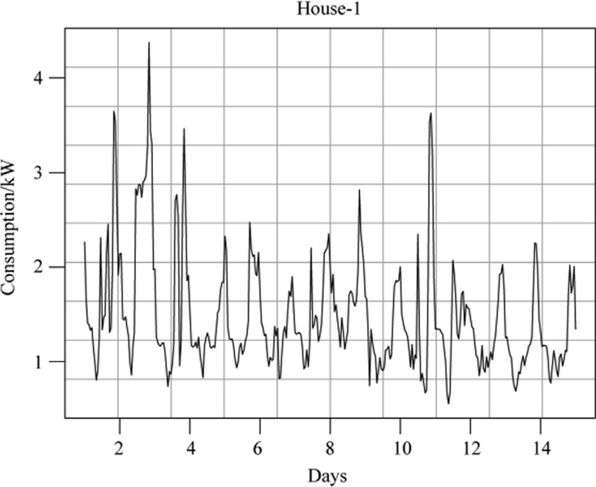
Fig. 1. Power consumption data of House-1 from July 15th to July 28th[13].

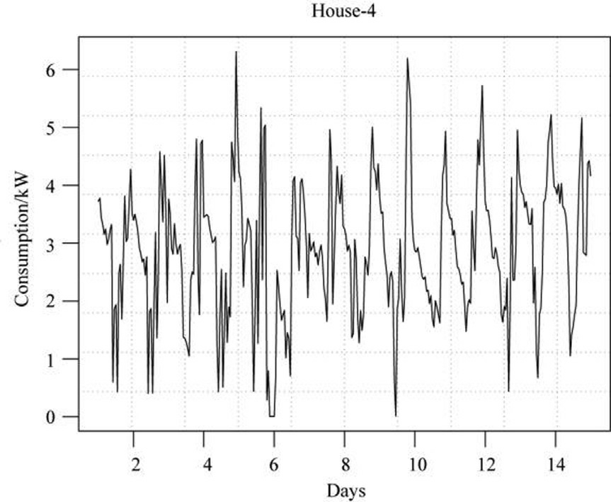
Fig. 2. Power consumption data of House-4 from June 1st to June 14th[13].

An AR based stochastic model of power consumption provides the current power consumption, for instance at time t, through a linear combination of p past consumption values, and the stochasticity in the prediction is modeled by adding an outcome of a stochastic variable εt.This forms a pth order AR model, represented as AR p ,given as foll ows:

where yt yt 1 y t pare the consumption values at the time t t 1 t p respect ively. ϕ1 ϕ2 ϕpare the AR coefficients. εtis modelled as white noise with zero mean and standard deviation of value one. cis a constant and it is obtained by taking the expected value of yt in(1):

For a stationary AR process, the expected value of the series remains constant over time, such that E yt E yt 1 μ,Since the expected value of the white-noise error is zero, E εt 0,substituting these conditions in the equation having expected values of ytyields,μ c ϕ1 ϕ2 ϕp μ,therefore, by rearranging the expression c μ ϕ1 ϕ2 ϕp μ,we have obtained the final equati on for the constant c:

where μ is the mean of the power consumption, around which a stationary time series fluctuates. The intercept c is mathematically linked to this mean that ensu res the AR process reproduces the correct average behavior. We introduce a backshift operator, B, which is defined as,Byt yt 1 B2 yt yt 2 and Bk yt yt k.The power of the backshift operator signifies the number of backshifts in the time series da ta. With the help of this operator, a simplified expression of (1) can be built as follows:

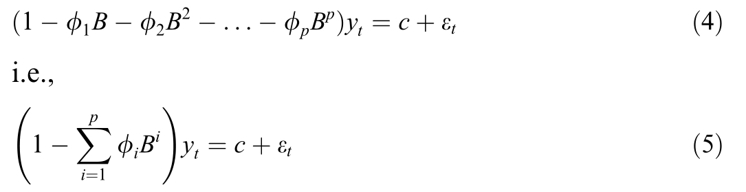
A compact representation is given as follows,

Similarly, an MA model provides an output by considering the current value of a time series (e.g., the stochastic error term εt)and a linear combination of the pa st values of the series. The qthorder MA model is represented by MA qand is given as follows:

It can be written with the backshift ope rator,B,as follows:

A compact representation is given as follows:

where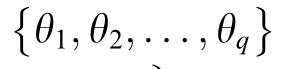are the MA coefficients and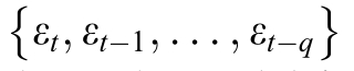are the current and lagged error terms.ARMA model is formed by the combination of autoregressive and moving average models. ARMA models (like AR and MA) consider that the given time series is stationary.The ARMA model is denoted by ARMA pq.p is the order of the AR component and q is the order of the MA component. The model is given as follows:

The assumption of stationarity of a given time series in an ARMA based model does not necessarily suit every application. To address this, autoregressive integrated moving average (ARIMA) model is also available in the literature.ARIMA is similar to ARMA model but the only difference is that it can a ccommodate the non-stationarity in time series by taking the difference ‘‘I”of the series to make it stationary. Differencing of order ‘‘d” can be defined as1 B d.In general,ARIMA model can be written as:

where is the first order differenced series, which can be mathematically represented as:

Similarly, second order differenced series can be mathematically represented as:  yt 2yt 1 yt 2. In general, the dth order differenced series can be represented as:The ARIMA model is denoted by ARIMA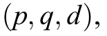where p is the order of AR component,d is the order of differencing,q is the order of the MA component,and c is the constant given in (2).

2.3 SARIMA based time series stochastic model

The seasonal autoregressive integrated moving average(SARIMA) model is an extension of the ARIMA model with an additional seasonal component. In time seri es,seasonality is the regular pattern of changes that repeat its cycle after ‘‘s” time steps [7]. The seasonal difference is the difference between the value and the value with its periodic lag, which is the multiple of ‘‘s”, for example, if we have a monthly data of energy consumption then s will be equal to 12 and the seasonal difference in this case will be.Similarly, if we have hourly data of energy consumption then s will be 24 and the seasonal difference for this case will beSeasonal differencing is used in order to remove the nonstationarity caused by the seasonal trends in the data.The shorthand notation to represent the SARIMA model which incorporates both the seasonal and non-seasonal components is as follows,

where p, d and q are the order of non-seasonal components, and P, D and Q are the order of seasonal components with the time period of repeated seasonal patterns s. Generally, SARIMA model can be written in a multiplicative form such as the seasonal and non-seasonal AR part should be mult iplied with each other on the lefthand side of the equation along with seasonal and nonseasonal differencing parts. Moreover, the seasonal and non-seasonal MA parts should be multiplied with each other on the right-hand side of the equation [34], i.e.,

SARIMA includes pth order non-seasonal autoregressive component (AR) that is Similarly, seasonal autoregressive component (SAR) is represented by with order P at lag s. The non-seasonal moving average an d seasonal moving average components are represented byof order q an d similarlyof order Q at lag s respectively. Finally, the non-seasonal and seasonal differencing of the SARIMA is repres ented by 1 B dof order d and 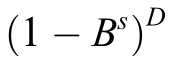of order D at lag s respectively [35].

2.4 SARIMA and ARIMA based model development for load prediction

This section briefly discusses the model development of the power consumption of residential buildings.Times series modeling incorporates three major steps:

1) Exploration of the time series data.

2) Model identification and coeffici ent estimation.

3) Model validati on.

In the first step of data exploration, we observe the data by constructing a time plot of the data and search for patterns and anomalies. We can visualize and identify different components of time series, e.g., trend, seasonal, and random noise components. Decomposition of time series data (see Fig. 3) can be achieved by multiplicative model because the dataset changes its values at every instant of time. A multiplicative model is given as follows:

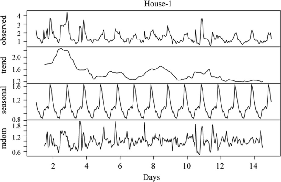
Fig. 3. Time series components for power consumption data of House-1.

where, yt is the given series Tt is the trend component, St is the seasonal component and Rt is the noise component.The trend component can be estimated by smoothing procedure e.g., moving averages, then series has to be detrended by dividing with trend component values. Seasonal component is estimated by taking the average of de-trended values in the series for a given seasonal period i.e., 24 hourly period. The random or noise component which can be extracted by dividing the series with the product of trend and seasonal component values[14]. Once we discover the patterns in the time series, the next step is to check whether the time series is stationary or nonstationary. Stationary is crucial in time series analysis because most of the analytical tools and models rely on it. For that, we perform the statistical test: augmented dickey fuller test (ADF), which evaluates the existence of unit root where unit root signifies the time series to be non-stationary and with the help of ADF test we can identify either the time series is stationary or non-stationary the relevant details can be found in ADF.

The second step performs the model identification,where we have to find the model orders and estimate unknown parameters. For ARIMA and SARIMA models,we find the orders for non-seasonal and seasonal autoregressive an d moving average components, i.e., (p,q,d)and (P,Q,D). To achieve this, we used the Hyndman-Khandakar. algorithm [36], which also considers the presence of unit roots in time series, similar to the ADF test,however, the algorithm also uses corrected akaike information criteria (AICc) to obtain the corresponding ARIMA and SARIMA model orders. Brief details of AICc are given in Appendix B.

We performed forecasting by employing the Hyndman-Khandakar algorithm. The procedure integrates conventional 5%-unit root testing to check whether the series is stationary or non-stationary, if unit root exist or null hypothesis is (p-value ＜ 0.05), then stationarity is rejected and non-seasonal differencing is applied with the order constrained d ‘‘2 to remove the trends from time series data. In the next step, the Seasonal Differencing (D ‘‘1)is applied only when seasonal unit roots indicate that the repeating seasonal pattern is non stationary. Stepwise exploration of autoregressive (AR) and moving average(MA) terms are evaluated, and optimal model order is selected by minimizing the corrected Akaike Information Criterion (AICc) to avoid overfitting. We specifically kept the Seasonal periods of 24 and 72 h to match forecasting horizons, and at last all the coefficients, including AR (p,P) and MA (q, Q) terms for both seasonal and nonseasonal components, as well as residual variance are estimated using maximum likelihood estimation(MLE)where principally we minimize the sum of the squared errors as follows,

where represents the predicted output at time t, which can be obtained e.g., for MA model in (8), for ARMA model in(11), for ARIMA model in(12) and for SARIMA model in (14). At the end we finally evaluate the residuals and observe whet her they are independent and identically distributed [14]. When the model identification and coeffi-cient estimation is done the identified model is then validated on a validation dataset. The model performance is measured using the metrics: root mean square error(RMSE) and mean absolute error (MAE) [37]. RMSE is given as,

MAE is given by,

This framework yielded ARIMA and SARIMA models that reliably captured both stochastic and seasonal dynamics of household electricity demand by ensuring reproducibility.

3 Case study

This section reports the simulation study carried out on the short term electric power demand of residential buildings in Lahore, Pakistan. All modelling and forecasting experiments were performed in R, and the forecasts were generated with classical ARIMA and SARIMA models.We monitored total of 41 houses at an hourly resolution.The electricity consumption data, originally recorded at one-minute intervals in kilowatts (kW), were resampled to an hourly resolution by averaging all measurements within each hour. This pre-processing procedure preserves the representative hourly load profile while maintaining the integrity of the demand patterns.

For brevity, the discussion below focuses on two representative houses (House-1 and House-4), while the aggregated numerical results for all dwellings are summarized later in Table 1 (see Appendix A).

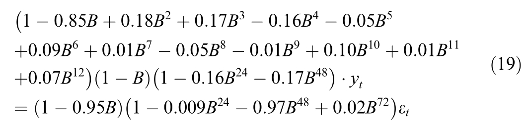
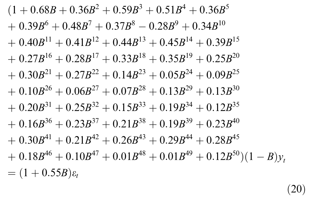
Two forecast horizons are considered: one day ahead(24 h) and three days ahead (72 h). The forecasts for all the houses (actual and predicted) are given in Fig. 11(Appendix C). The models were trained on the most recent 14 days of observations. Fig. 4 presents the short-term power consumption forecasts for House-1 using the fitted models including the already described ARIMA(50,1,1)and SARIMAshowing the predicted values over 24 h (left) and 72 h (right). Consistent with the information criteria thethe seasonal model achieves lower forecast errors and is structurally more compact,making it preferable for downstream control tasks. Both models follow the load trend well during the first 40 h;however, a sharp and unanticipated peak between hours 40 and 50 is missed. Forecasts for the remaining period(hours 50-70) closely match the actual trajectory.

SARIMA model.

ARIMA model.

For House--4, the training window is likewise 14 days.The fitted models are SARIMAand ARIMA(60,0,0). Fig. 5 shows their forecasts for both the 24 h (left) and 72 h (right) horizons. Despi te having identical model orders, the seasonal specification is significantly more concise AIC,cSARIMA 7 84vs 881 and therefore preferable for real time deployment and therefore preferable for real time deployment.

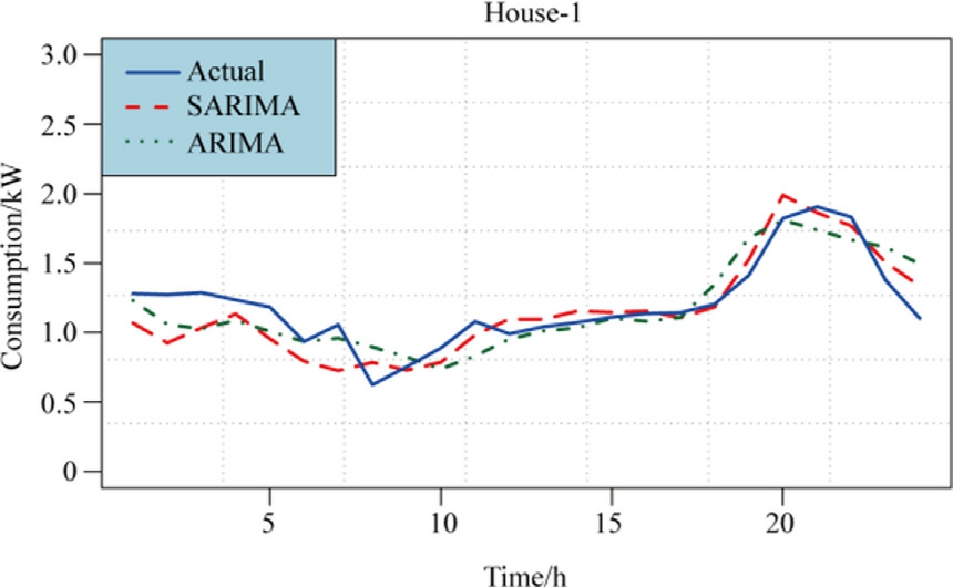
Fig. 4. House-1: 24 h forecast (left) and 72 h forecast (right).

SARIMA model.

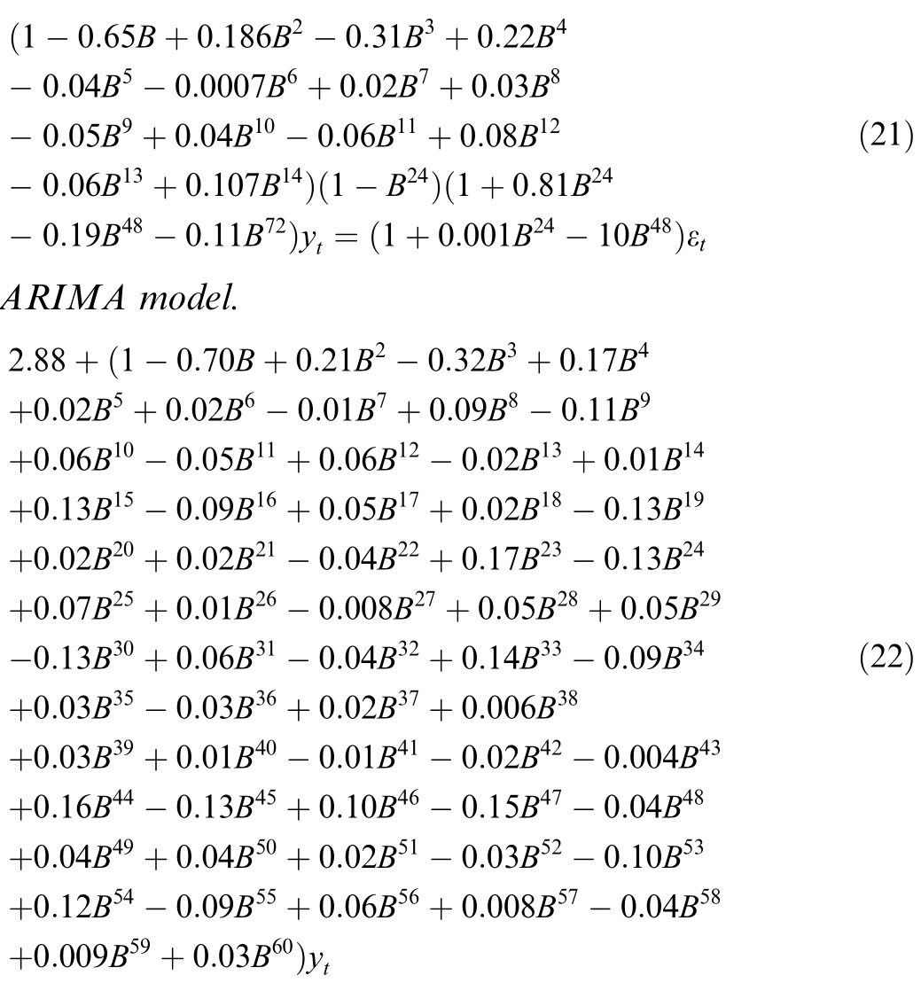
In evaluating forecasting models, both ARIMA and SARIMA were applied to the Lahore household dataset, and the comparative evidence in Table 1 of Appendix A demonstrates SARIMA’s consistent superiority across both short (24 h) and long (72 h) horizons. While ARIMA is traditionally suited for non-seasonal data, its neglect of recurring cycles led to higher model orders, higher forecast errors, and weaker fit. SARIMA, by embedding seasonal differencing and seasonal autoregressive/moving average terms, captured subtle daily and weekly patterns that ARIMA could not, yielding lower RMSE and MAE values (e.g., House-4, House-15, House-16), more parsimonious specifications (e.g., House-1, House-2, House-7),and consistently reduced AICc scores across households.Structurally, SARIMA uses seasonal terms, reducing reliance on high non-seasonal orders and enhancing interpretability and computational efficiency. Practically, this translates into forecasts that are more accurate, stable,and scalable,enabling power sectors to anticipate demand peaks,allocate resources effectively,and mitigate blackout risks.

4 Clustering of residenti al buildings

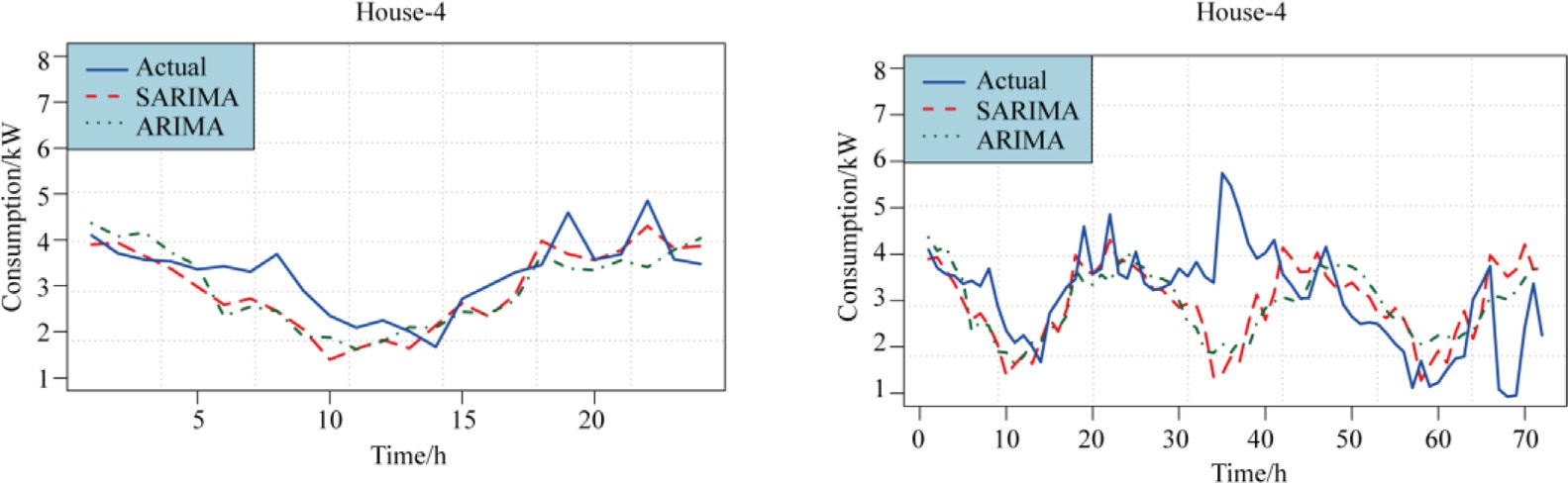
Fig. 5. House-4: 24 h forecast (left) and 72 h forecast (right).

In this paper clustering of residential buildings has been performed by using machine learning algorithm that is hierarchical clustering. The aim of clustering is to group the residential buildings based on their power consumption values along with additional physical attributes physical attributes which have been listed in Table 2 (Appendix A). Moreover, it can help the power companies to provide information about the groups of houses that are similar in electricity consumption with their physical parameters.Data set for clustering contains 42 residential buildings,to analyze the behavior of the occupants and their electricity consumption patterns, four different sets of grouping is performed with summer, autumn, winter and spring seasons power consumption along with additional physical features. Hierarchical clustering is one of the simplest unsupervised learning methods in which clusters are to be made on the basis of a distance matrix which is computed by Euclidean distance matrix for every season and is given as,

Four different seasons for clustering are taken into account to predict the behavior of individual houses power consumption. In the following sub-sections, we present the season-wise clustering results to analyze variations in household electricity usage patterns.

4.1 Summer season clustering

For summer season, the clusters are formed using the electricity consumption data of residential buildi ngs in summer season specifically, along with physical parameters.

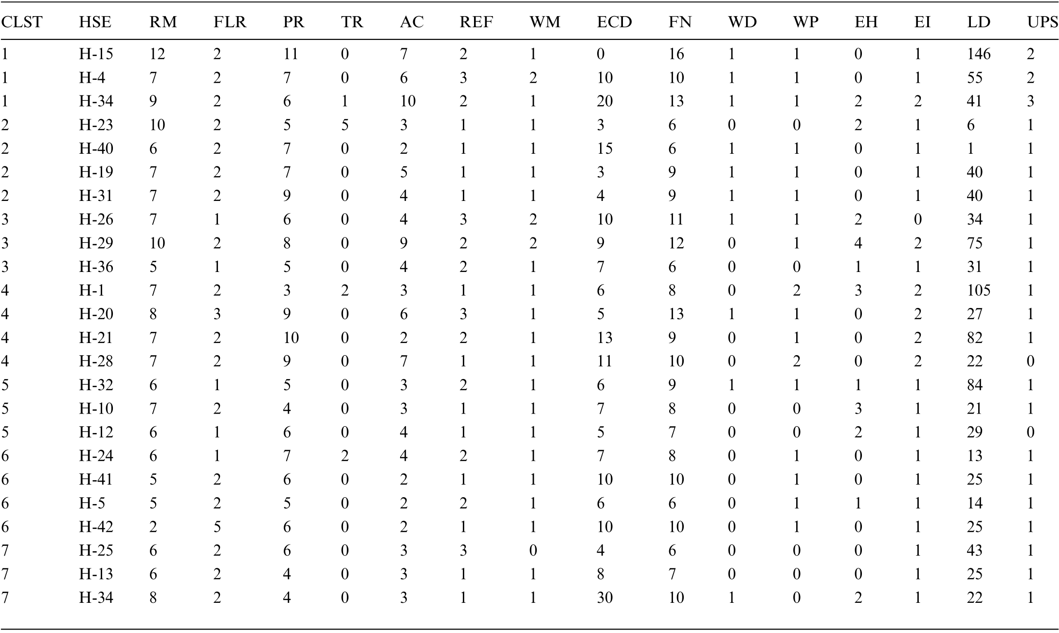
Which is represented in Fig. 6 by the cluster dendrogram. On the vertical axis height represents the values of distance matrix computed by Euclidean distance formula in hierarchical clustering method and horizontal axis represents the number of houses. Lower value of height represents high similarity among the houses and high value of height represents low similarity among different houses.In the proposed work, we have represented the results of seven different clusters formed by the combination of electricity consumption of summer season and their physical parameters e.g., no of rooms, floor, occupants, and total no of electricity devices. Fig. 6 represents the clusters of summer season based on both electricity consumption and physical parameters of the houses, similarly the separate analysis of different physical parameters used in houses are listed in Table 3 (Appendix A) which are grouped into seven different clusters.

4.2 Autumn season clustering

Following the analysis of the summer season, Fig. 7 represents the clustering result for the electricity consumption of autumn season for different groups of houses and their physical parameters are represented in Table 4(Appendix A).

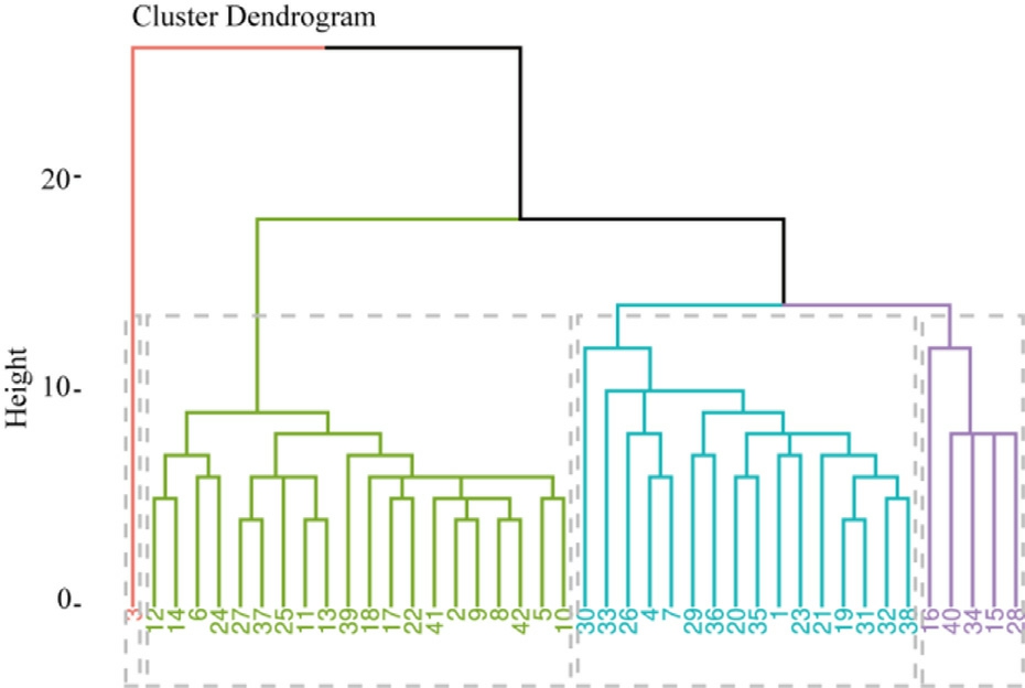
Fig. 6. Hierarchical clustering with summer season electricity consumption.

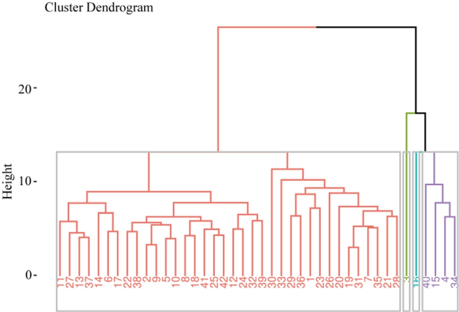
Fig. 7. Hierarchical clustering with autumn season electricity consumption.

4.3 Winter season clustering

To examine seasonal patterns for winter, Figure Fig. 8 displays the clustering outcomes based on winter electricity consumption, incorporating phy sical characteristics of the residential buildings. Table 5 (Appendix A) provides a detailed summary of these attributes for each cluster.

4.4 Spring season clustering

The final seasonal clustering, shown in Fig. 9, depicts the spring-time consumption behaviors alongside household physical features while Table 6 (Appendix A) complements this analysis by summarizing the attributes used to form the residential groups.

The hierarchical clustering analysis grouped households into archetypal consumption profiles based on seasonal demand, appliance ownership, and occupancy patterns.These clusters reveal distinct behavioral patterns, some households exhibit high evening peaks driven by cooling and lighting loads, while others show lower electricity consumption profiles associated with smaller family sizes or fewer appliances. From a demand-side management perspective, these insights are critical. By identifying clusters of households with similar load characteristics, power sectors can design different strategies rather than applying uniform interventions. For example, households with high electricity consumption-profile can be targeted with demand response pro-grams that incentivize load shif ting from peak to off-peak hours, while low electricity consumption-profile households may benefit more from energy efficiency measures. Practically, this enables power sectors to anticipate demand surges more precisely, allocate resources efficiently,and tailor interventions to household types. The house-holds belonging to highconsumption clusters can be prioritized for load shifting during peak hours, while low-consumption clusters can be leveraged for stability. In rapidly urbanizing regions such as Lahore, where grid stress and blackout risks are prevalent, clustering ultimately provides a scalable framework for personalized demand-side management.

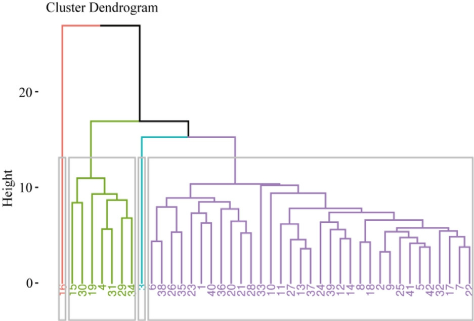
Fig. 8. Hierarchical clustering with winter season electricity consumption.

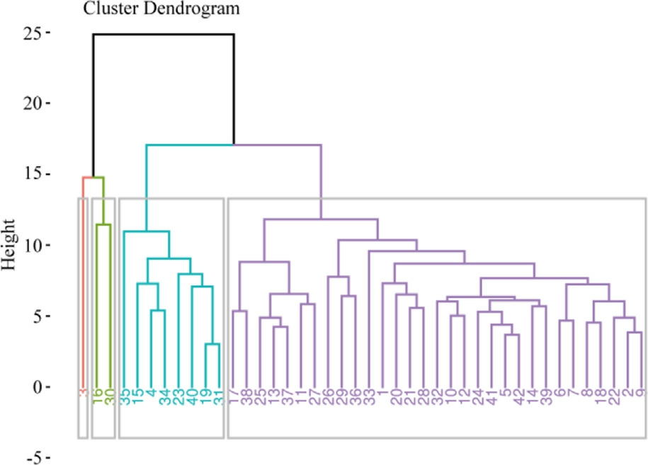
Fig. 9. Hierarchical clustering with spring season electricity consumption.

5 Dis cussion

The case study and results presented in this paper underscore several key contributions and implications for both research and practice in residential electricity forecasting in developing nations.

1) Presents a rare instance of high-resolution,household-level electricity forecasting in the Global South, using detailed data collected from homes in Lahore, Pakistan.

2) Conducts a comparative evaluation of classical time series models, demonstrating how seasonal extensions like SARIMA outperforms ARIMA in capturing residential demand patterns.

3)Combines short-term forecasting with clustering informed by both temporal usage profiles and household characteristics, allowing for more contextaware and group-specific insights into energy consumption.

We observed that across all houses, the SARIMA models consistently outperformed ARIMA models in terms of accuracy and parsimony.As reported in Table 1 in Appendix A, SARIMA achieved lower RMSE and MAE values for the majority of cases. For example, House-1 showed a reduction in AICc from 251 (ARIMA) to 229 (SARIMA),while maintaining tighter tracking of consumption spikes.The seasonal models also required fewer coefficients than their ARIMA counterparts (e.g., 12 vs. 50 autoregressive terms in House-1), making them better suited for embedded or real-time applications. This performance highlights the importance of accounting for seasonal structures—such as daily or weekly consumption cycles—in residential load forecasting. By explicitly modeling these recurring patterns, SARIMA can offer more reliable and interpretable predictions, especially in households where lifestyle-driven consumption patterns recur over time.

The clustering analysis revealed natural groupings of households with similar seasonal demand patterns and appliance ownership. For instance, homes with higher air conditioner counts or larger household sizes tended to cluster together,particularly in the summer season. This clustering supports demand-side strategies such as load shifting or targeted energy-efficiency programs. Furthermore, clustering allows grid operators and power companies to design tailored interventions by targeting specific con sumer archetypes rather than relying on generic consumption profiles.For example, clusters representing high-load households with large families can be targeted for smart metering or incentive-based load control, while low-load clusters may be better served through awareness campaigns.

This study demonstrates that accurate short-term residential forecasting is feasible using lightweight time series models even in id="generateCatalog_21" style="text-align: left; text-indent: 0em; font-size: 1.4em; color: rgb(195, 101, 0); font-weight: bold; margin: 0.7em 0em;">6 Conc lusion

This paper presented a framework for modeling shortterm electricity consumption across 41 individual residential buildings in Lahore, Pakistan. The proposed methodology applies class ical time series techniques to capture varying consumption behaviors shaped by occupant activity and seasonal trends.

Given the limited availability and periodic nature of high-resolution household data, ARIMA and SARIMA models were implemented to forecast electricity demand for the next 24 and 72 h. The comparative analysis revealed that SARIMA generally outperformed ARIMA,achieving lower errors across both horizons: for the 24-h forecast, SARIMA reduced the MAE value from 0.30 kW to 0.23 kW and RMSE value from 0.40 KW to 0.32 kW;for the 72-h forecast,MAE value decreased from 0.39 kW to 0.350 kW and RMSE value from 0.51 kW to 0.41 kW. In addition, the MAPE results further support the superiority of SARIMA, with error values decreasing from 36.9% to 28.3% for the 24-h horizon and from 49.1% to 39.54% for the 72-h horizon. These results demonstrate SARIMA’s superior ability to capture both stochastic and seasonal patterns in household electricity demand (Fig. 10).

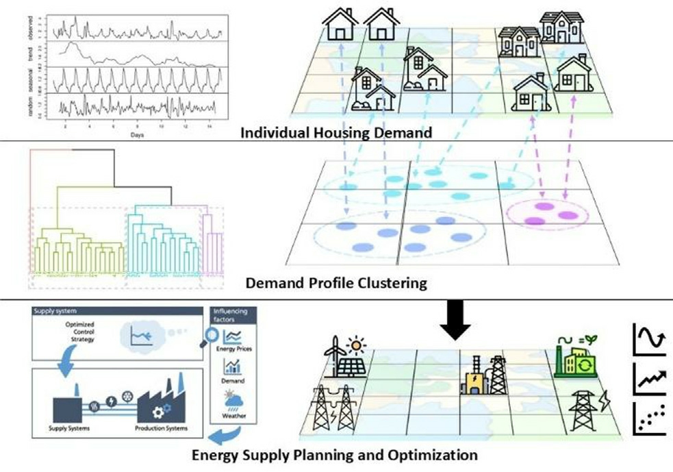
Fig. 10. SARIMA-based household electricity demand forecast ing,clustering and energy optimization.

Moreover, SARIMA requires fewer model parameters—resulting in reduced computational overhead. These short-term forecasts can support demand-side management strategies and help ensure more reliable electricity delivery. In addition, clustering of households based on both electricity consumption patterns and physical attributes enabled the identification of behavioral similarities among households. The clustering was validated using silhouette widths ranging from 0.13 to 0.25, supporting the reliability of the identified household groups. This grouping can help power companies better target demand-side interventions, anticipate peak loads, and reduce the risk of blackouts.

CRediT authorship contribution statement

Sana Arif: Writing - original draft, Visualization,Methodology, Investigation, Formal analysis, Data curation, Conceptualization. Rabbia Hassan: Writing - review& editing. Hasan Arshad Nasir: Validation, co-supervision.Naveed Riaz: Revi ew & editing, Validation. Imran Mahmood: Writing - original draft, Methodology, Investigation, Formal analysis, Conceptualization, Supervision,Project administration.

Declaration of competing interest

The authors declare that they have no known competing financial interests or personal relationships that could have appeared to influence the work reported in this paper.

Appendix A

Table 1

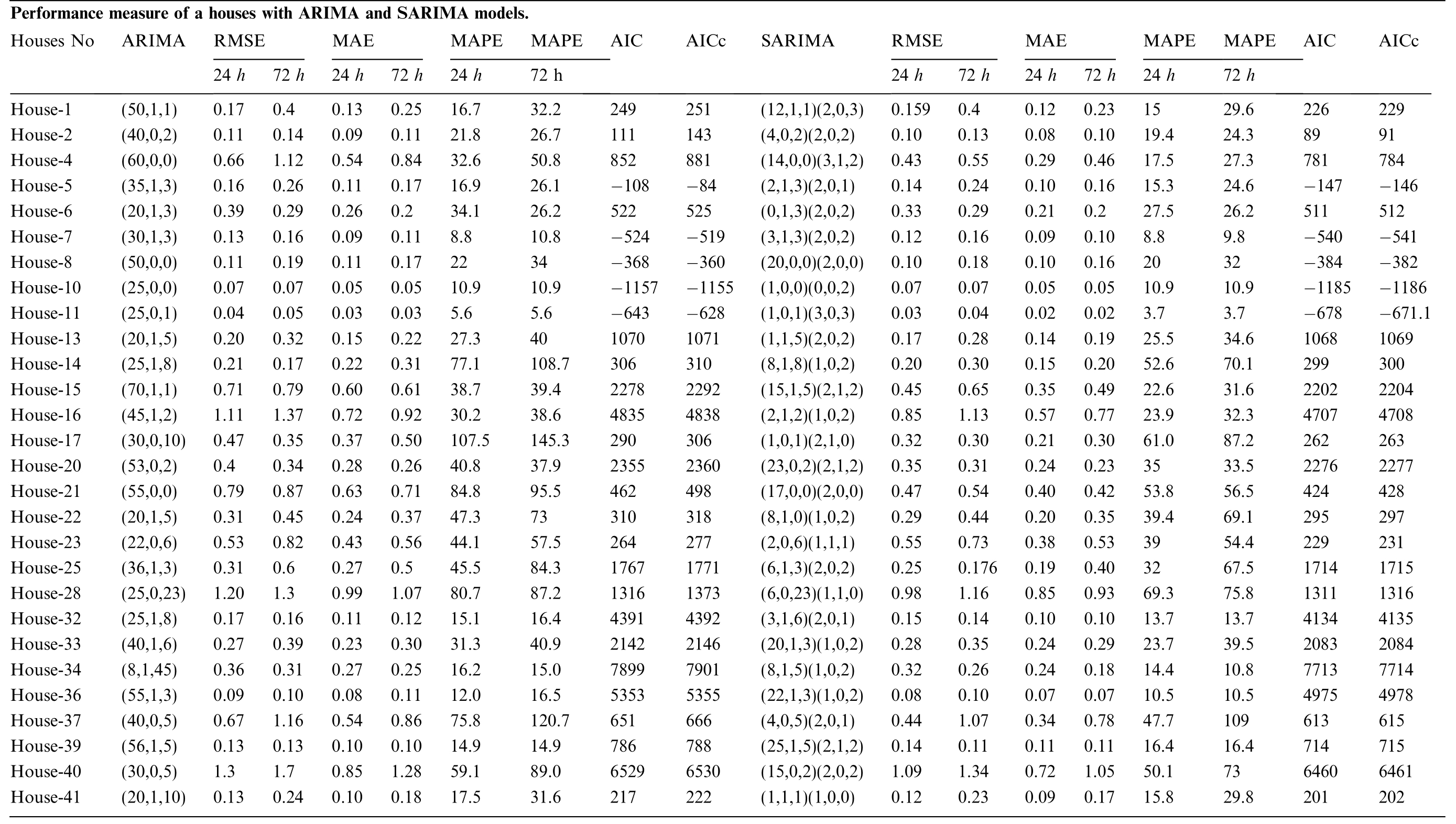
Table 2 Physical parameters.

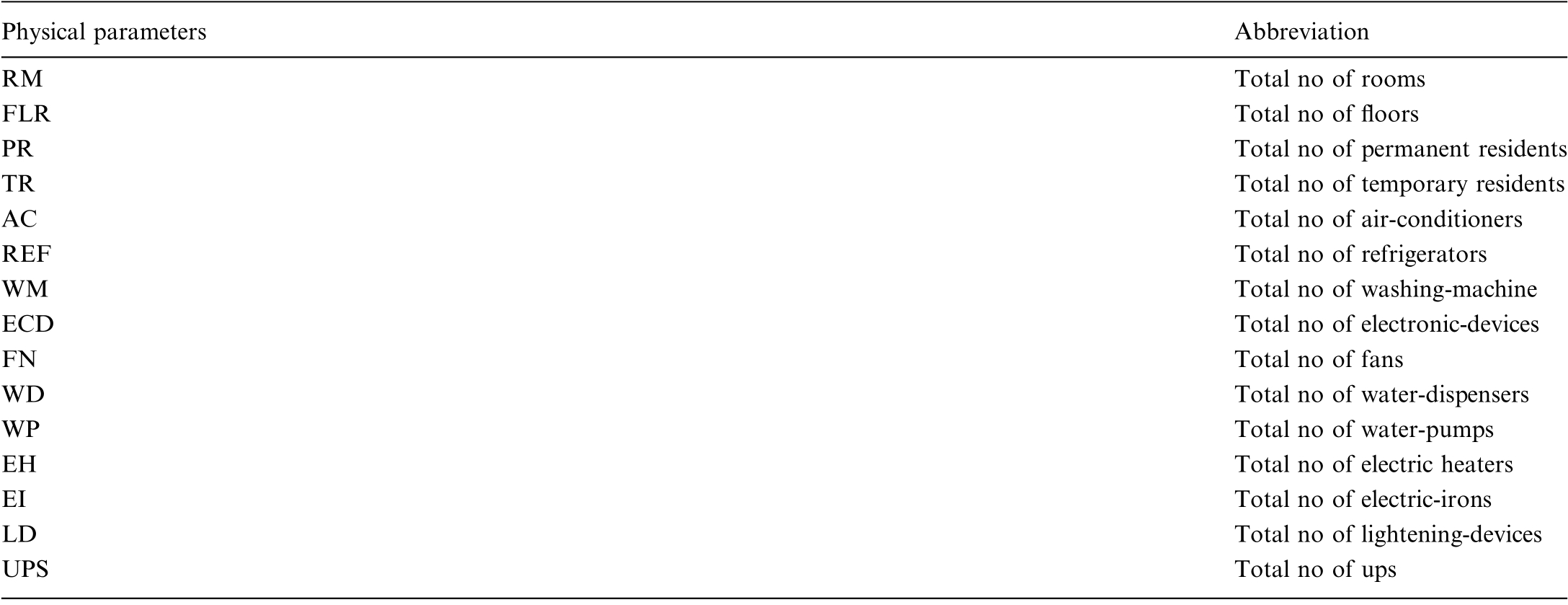
Table 3 Clustering of summer season power consumption and physical parameters.

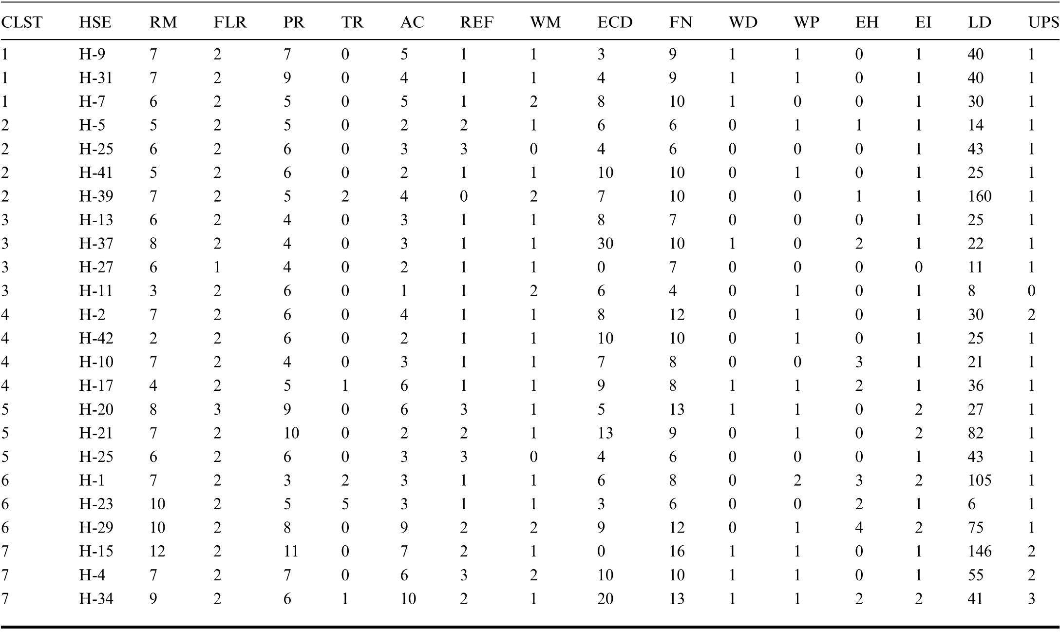
Table 4 Clustering of autumn season power consumption and physical parameters.

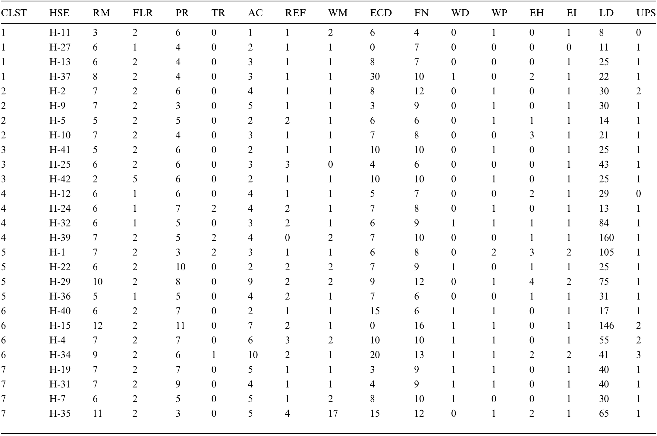
Table 5 Clustering of winter season power consumption and physical parameters.

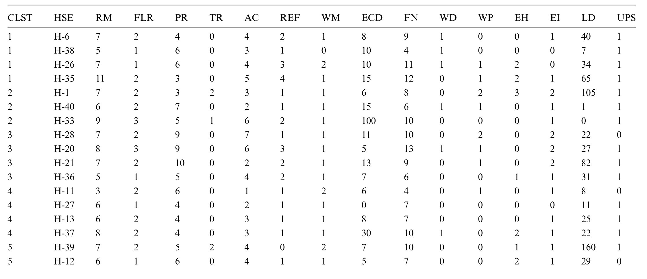
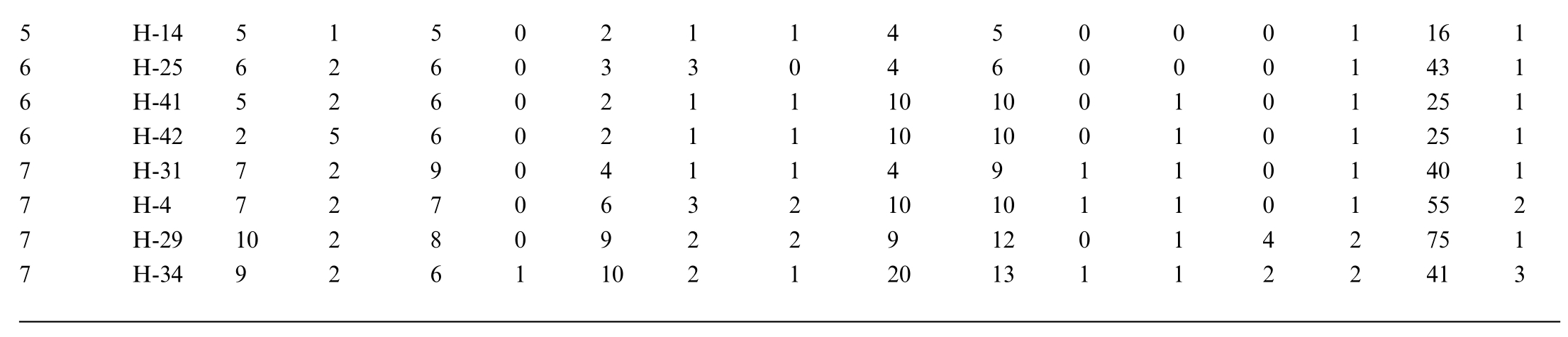
Table 6 Clustering of spring season power consumption and physical parameters.

Appendix B

Akaike Information Criteria (AIC) is used for determining the orders of ARIMA and SARIMA models. Basic formula used to compute the AIC for ARIMA model is,where k is the intercept of the ARIMA model (i.e., the mean of the series) e.g.,k = 1when the constant term in AR IMA and SARIMA models then there is an intercept in the ARIMA and SARIMA models and k = 0when constant in

ARIMA and SARIMA models 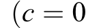there is no intercept in the ARIMA and SARIMA models whereas L is the likelihood of the data which is estimated by maximum likelihood estimation by minimizing the sum of squared errors i.e.,.

Similarly for the SARIMA model, AIC is represented as:the value of 1 is added because variance is estimated for the AR,MA, SAR and SMA components. Similarly, L is the loglikelihood estimate that measures the model fit whereas lower the value of AIC indicates better model fitting.When sample size or number of observations i.e., T is small then there is a probability that AIC will overfit the model, to overcome that corrected akaike information criteria AICc is preferred instead of AIC value in order to compute better model orders for ARIMA and SARIMA.AICc is represented mathematically as:

where, m comprises the number of ARIMA and SARIMA model parameters such as:,T is the total number of observations in the series and kis the intercept of the ARIMA and SARIMA model [14].

Appendix C

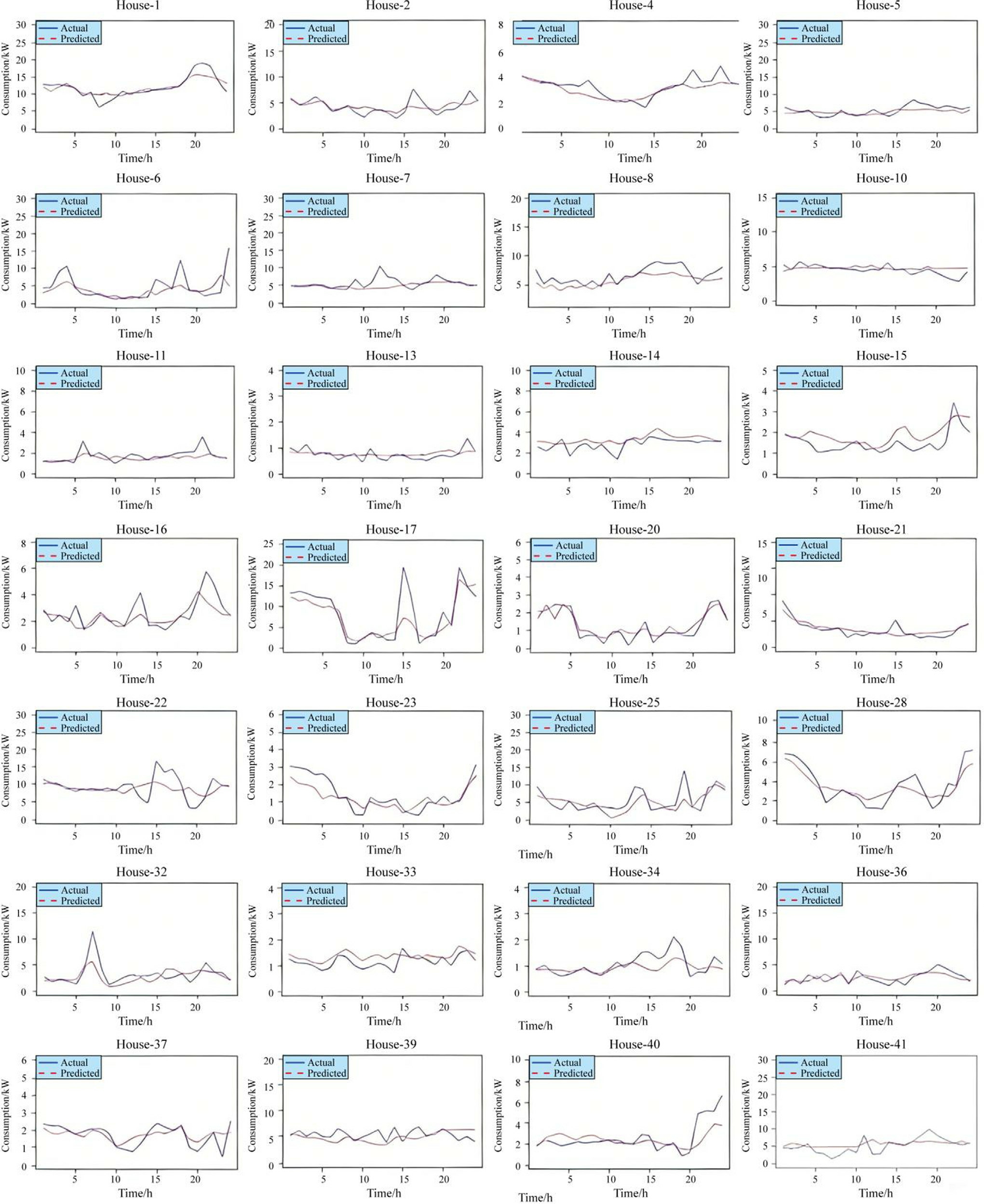
Fig. 11. Comparison of Actual and Predicted Consumptions-41 houses (24 h).

References

[1]M.A.M. Daut, M.Y. Hassan, H. Abdullah, et al., Building electrical energy consumption forecasting analysis using conventional and artificial intelligence methods: a review, Renew.Sustain. Energy Rev. 70 (2017) 1108-1118.

[2]H. Zhao, F. Magoule`s, A review on the prediction of building energy consumption, Renew. Sustain. Energy Rev. 16 (6) (2012)3586-3592.

[3]C. Kuster, Y. Rezgui, M. Mourshed, Electrical load forecasting models: a critical systematic review, Sustain. Cities Soc. 35 (2017)257-270.

[4]C. Deb, F. Zhang, J. Yang, et al., A review on time series forecasting techniques for building energy consumption, Renew.Sustain. Energy Rev. 74 (2017) 902-924.

[5]Y. Kim, H. Son, S. Kim, Short-term electricity load forecasting for institutional buildings, Energy Rep. 5 (2019) 1270-1280.

[6]F. Yasmeen, M. Sharif, Forecasti ng electricity consumption for Pakistan, Int. J. Emerg. Technol. Adv. Eng. 4 (4) (2014) 496-503.

[7]X. Chang, M. Gao, Y. Wang, X. Hou, Seasonal autoregressive integrated moving average model for precipitat ion time series, J.Math. Stat. 8 (4) (2012) 500-505.

[8]L.G. Swan, V.I. Ugursal, Modeling of end-use energy consumption in the residential sector: a review of modeling techniques, Renew.Sustain. Energy Rev. 13 (8) (2009) 1819-1835.

[9]I. Mahmood, N.H.A. Quair-tul-ain, et al., A hierarchical multiresolution agent-based modeling and simulation framework for household electricity demand profile, SIMULATION 96(8)(2020)655-678.

[10]S. Fan, R.J. Hyndman, Short-term load forecasting based on a semi-parametric additive model, IEEE Trans. Power Syst. 27 (1)(2011) 134-141.

[11]K. Chen, K. Chen, Q. Wang, et al., Short-term load forecasting with deep residual networks, IEEE Trans. Smart Grid 10(4)(2019)3943-3952.

[12]N. Charlton, C. Singleton, A refined parametric model for shortterm load forecasting, Int. J. Forecast. 30 (2) (2014) 364-368.

[13]A. Nadeem, N. Arshad, PRECON: Pakistan residential electricity consumption dataset. In: Proceedings of the Tenth ACM Internatio nal Conference on Future Energy Systems, Phoenix,AZ, USA, 25-28 June 2019, 2019, pp. 52-57.

[14]R.J. Hyndman, G. Athanasopoulos, Forecasting: Principles and Practice, second ed., OTexts, Melbourne, 2018.

[15]R. Granell, C.J. Axon, D.C.H. Wallom, Clustering disaggregated load profiles using a Dirichlet process mixture model, Energ.Conver. Manage. 92 (2015) 507-516.

[16]M. Azaza, F. Wallin, Smart meter data clustering using consumption indicators: responsibility factor and consumption variability. In: 9th Internationa l Conference on Applied Energy(ICAE 2017), Cardiff, UK, 21-24 August 2017, Energy Procedia,2017, 142, pp. 2236-2242.

[17]P. Chujai, N. Kerdprasop, K. Kerdprasop, Time series analysis of household electric consumption with ARIMA and ARMA models.In: Proceedings of the International Multi Conference of Engineers and Computer Scientists 2013, vol. I, Hong Kong, 13-15 March 2013, 2013, pp. 295-300.

[18]P. Ma, S. Cui, M. Chen, et al., Review of family-level short-term load forecasting and its application in household energy management system, Energies 16 (15) (2023) 5809.

[19]Newsham G R, Birt B J (2010) Building-level occupancy data to improve ARIMA-based electricity use forecasts.In:Proceedings of the 2nd ACM Workshop on Embedded Sensing Systems for Energy-Efficiency in Buildings, Zurich, Switzerland, 2 November 2010, pp 13-18.

[20]X.M. Zhang, K. Grolinger, M.A.M. Capretz, Forecasting residential energy consumption using support vector regressions.In: Proceedings of the IEEE International Conference on Machine Learning and Applications, Orlando, FL, USA, December 2018.

[21]R.V. Klyuev, I.D. Morgoev, A.D. Morgoeva, et al., Methods of forecasting electric energy consumption: a literature review,Energies 15 (23) (2022) 8919.

[22]P. Hasanah, C.A. Sari, S.A.W. Dinata,Electricity load forecasting in East Kalimantan on religious holidays using SARIMA,Math.J.Model. Forecast. 1 (2) (2023) 54-64.

[23]S. Zhao, Urban electricity consumption forecasting based on SARIMA and random forest modeling, J.Electrotechnol.Electric.Eng. Manage. 7 (1) (2024) 113-118.

[24]C. Yin, K. Liu, Q. Zhang, et al., SARIMA-based medium- and long-term load forecasting, Strategic Plann. Energy Environ.42(2)(2023) 283-306.

[25]A. Akso¨z, S. Oyucu, E. Bicer, R. Bayındır, Analysis of SARIMA Models for Forecasting Electricity Demand. In: 12th International Conference on Smart Grid (icSmartGrid 2024), Setu´bal, Portugal,27-29 May 2024, pp. 767-771.

[26]M. Bilgili, E. Pinar, Gross electricity consumption forecasting using LSTM and SARIMA approaches: a case study of Tu¨rkiye,Energy 284 (2023) 128575.

[27]J.W. Chan, C.K. Yeo, A transformer-bas ed approach to electricity load forecasting, Electr. J. 37 (2) (2024) 107370.

[28]Y. Ning, R. Zhao, S. Wang, et al., Probabilistic short-term power load forecasting based on B-SCN, Energy Rep. 8 (2022) 646-655.

[29]S. Zeng, C. Liu, H. Zhang, et al., Short-Term load forecasting in power systems based on the prophet-BO-XGBoost model,Energies 18 (2) (2025) 227.

[30]G.J. Tsekouras, P.B. Kotoulas, C.D. Tsirekis, et al., A pattern recognition methodology for evaluation of load profiles and typical days of large electricity customers, Electr. Pow. Syst. Res. 78 (9)(2008) 1494-1510.

[31]G. Chicco, R. Napoli, F. Piglione, Comparisons among clustering techniques for electricity customer classification, IEEE Trans.Power Syst. 21 (2) (2006) 933-940.

[32]F. Rodrigues, J. Duarte, V. Figueired o, A comparative analysis of clustering algorithms applied to load profiling, in: P. Perner, A.Rosenfeld (Eds.), Machine Learning and Data Mining in Pattern Recognition. MLDM 2003. Lecture Notes in Computer Science,vol. 2734, Springer, Berlin, Heidelberg, 2003, pp. 73-85.

[33]C. Si, S. Xu, C. Wan, et al., Electric load clustering in smart grid:methodologies, applications, and future trends, J.Mod Power Syst.Clean Energy 9 (2) (2021) 237-252.

[34]L. Wiri, I.D. Essi, Seasonal Autoregressive Integrated moving Average (SARIMA) Modelling and forecasting of inflation rates in Nigerian (2003-2016), Int. J. Appl. Sci. Math. Theory 4 (1) (2018)1-14.

[35]T.W. Mapuwei, O. Bodhlyera, H. Mwambi,Univariate time series analysis of short-term forecasting horizons using artificial neural networks: the case of public ambulance emergency preparedness,J.Appl. Math. 2020 (2020) 1-11.

[36]R.J. Hyndman, Y. Khandakar, Automatic time series forecasting:the forecast package for R, J. Stat. Softw. 27 (3) (2008) 1-22.

[37]M.V. Shcherbakov, A. Brebels, N.L. Shcherbakova, e t al., A survey of forecast error measures, World Appl. Sci. J. 24 (24)(2013) 171-17 6.

Received 25 May 2025; re删vis除ed 26 March 2026; accepted 14 April 2026

Peer review under the responsibility of Global Energy Interconnection Group Co. Ltd.

* Corresponding author

at: School of Electrical Engineering and Computer Science (SEECS), National University of Sciences and Technology(NUST),Islamabad, Pakistan.

E-mail addresses: sarif.msee17seecs@seecs.edu.pk (S. Arif), rabbia.hassan@seecs.edu.pk (R. Hassan), hasan.nasir@seecs.edu.pk (H.A. Nasir), naveed.riaz@seecs.edu.pk (N. Riaz), imran.mahmood@seecs.edu.pk, imran.hashmi@cs.ox.ac.uk (I. Mahmood).

https://doi.org/10.1016/j.gloei.2026.04.001

2096-5117/© 2026 Global Energy Interconnection Group Co. Ltd. Publishing services by Elsevier B.V. on behalf of KeAi Communications Co. Ltd.This is an open access article under the CC BY-NC-ND license(http://creativecommons.org/licenses/by-nc-nd/4.0/).

Sana Arif received her bachelor’s degree in electrical engineering from Riphah International University, Islamabad, Pakistan, and her M.S. degree in Control Systems from the School of Electrical Engineering and Computer Science(SEECS), National University of Sciences and Technology (NUST), Islamabad, Pakistan. She currently serves as an Assistant Manager/Sub-Division Officer at Peshawar Electric Supply Company (PESCO), one of the distribution companies of Pakistan(DISCOS).Her research interests include control systems, power distribution system planning, and energy optimization.