0 Intr oduction

The adverse effects of using fossil fuels on the environment vary from climate change to water pollution [1].Therefore, the United Nations’ sustainable development goals (SDGs) urged the adoption of renewable energy under SDG 7 of the initiative. In Malaysia, the National Energy Transition Roadmap (NETR) sets a strategic plan to achieve net-zero emissions by 2050 and increa se Renewable Energy (RE) capacity to 70% by 2050 [2]. The key benefit of RE is its environmentally friendly nature and its beneficial role in reducing greenhouse gases [3]. However,implementing RE on a large scale entails inheren t risks due tothe different design architecture.

The current electrical grid system works by maintaining supply–demand balance, which translates to frequency stability. Synchronous generators (SG) play an important role in this process. SG operates by converting mechanical power to electrical power. This gives it an inherent inertia capability due to the stored energy in its rotating mass.Whereas it plays a crucial role when a large imbalance occurs in the system, called contingency. It helps mitigate the frequency drop by gradually decreasing it and, as a result, provides the system with sufficient time to respond and restore balance.Conversely,renewable energy sources such as solar photovoltaics (PV) lack rotating mass and hence do not contribute to inertia.RE’s inherent intermittent and unpredictable nature amplifies the power generation stability problem[4] and compounds the problem. As aresult of the reduced inertia, the power system will be more vulnerable to contingencies and possibly complete network blackouts. This problem is further exaggerated inthe increasingly interconnected power networks, where any contingency in one area can propagate to the other.

In the literature, tackling frequency regulation problems varies, as some studies focused on improving control ofpower plants through a process called load frequency control (LFC). Other studies focused on implementing energy storage devices (ESSs) to mitigate any imbalance and replicate an inertia-like response.

A set of papers focused on enhancing conventional PID controllers, contributing to load frequency control by using advanced tuning optimization or cascading the control.In[5], a PID controller of a single-area microgrid was tuned with artificial rabbit optimization. In [6], PID controllers were tuned with golden eagle optimization, and the testing power system was contrasted with the others byutilizing a four-area power network with three areas connected directly together and one area indirectly connected. Additionally, the system was equipped with HVDC lines. In [7], PID controllers were tuned with the Mayfly algorithm, and the power system used consisted ofa two-area model. In[8], pelican optimization was used for tuning PID controllers in a system consisting of four areas, each with a distinct generation type. In [9], a cascaded PI controller was proposed, consisting of PI-PD control. The parameters were tuned with the One-to-One-by-On e algorithm and were tested on a four-area interconnected power system. In [10], the PID controllers were extended to other partial fraction order controllers,including Tilt integral derivative (TID) controller and Fractional Order Proportional Integral Derivative(FOPID)controllers.In[10], jellyfish optimization was utilized for tuning the controller parameters in a three-area interconnected power system,and concluded the superiorityof TID controllers. Additionally, the papers started to shift to fractional-order controllers. In [11], a proposed new Tilt FOID controller for a two-area power syst em and the utilized imperial colonist algorithm.In[12], a cascaded TFOID controller with a PD controller with a filter was proposed and tuned with the artificial hummingbird algorithm. The syst em was a one-area grid model. Disturbance rejection control for LFC was also explored in [13]and [14]. In [13], active disturbance rejection control was utilized with a novel hybrid reinforcement-based memetic particle swarm optimization. The system utilized for testing consisted of two-area interconnected system with thermal power plants. As for [14], flatness-based active disturbance rejection control was utilized in two interconnected areas with thermal power plants. Fuzzy logic was also utilized in different types of controllers in [15,16],and [17]. In [15], interval type 2 fuzzy logic control was proposed for use in a two-area power system. In [16], a fuzzy logic PID controller was proposed in a twointerconnected-area power system.In[17], fuzzy logic sliding mode control was proposed for a single-area power system. Consequently, in [18] decentralized sliding mode control scheme was proposed for a four-area power system. In [19], a novel deep neural network controller was proposed for a two-area interconnected power system.Table 1 highlights all the distinct characteristics of each system used for testing.

Tackling the low inertia problem with improved LFC is essential and leveraging advancements in control technology. As for emulating inertia from ESS,it is a critical solution with the accelerating advancement in ESSs.

However, the literature does not address the variety of different power systems and interconnections that exist in power grids. Studies of interconnected power systems in general examine generalized theoretical models without consideration of possible real-life interconnections or the possible mix of generation types. Furthermore, there have been no extensive studies on how frequency instability propagates through different areas. More notably, the solution given to the problem is focused on improving the control instead of in which power system area is most applicable. Understanding the unique connections and how disturbances propagate across them is crucial, as it enables better formulation of solutions to the low-inertia problem.

This paper’s contributions lie in modeling a dynamic frequency response model based on the peninsula of Malaysia, consisting of four unique interconnected areas,tostudy the effects of the propagating low inertia and increased RE adoption in the system during regionspecific disturbance. The uniqueness of the system relies onits diverse conventional generation types and the adoption ofRE.Furthermore,thepaper proposes them FDmetricto measurethe frequencynadir sensitivitytodifferent contingency levels.

Table 1 Load frequency control papers.

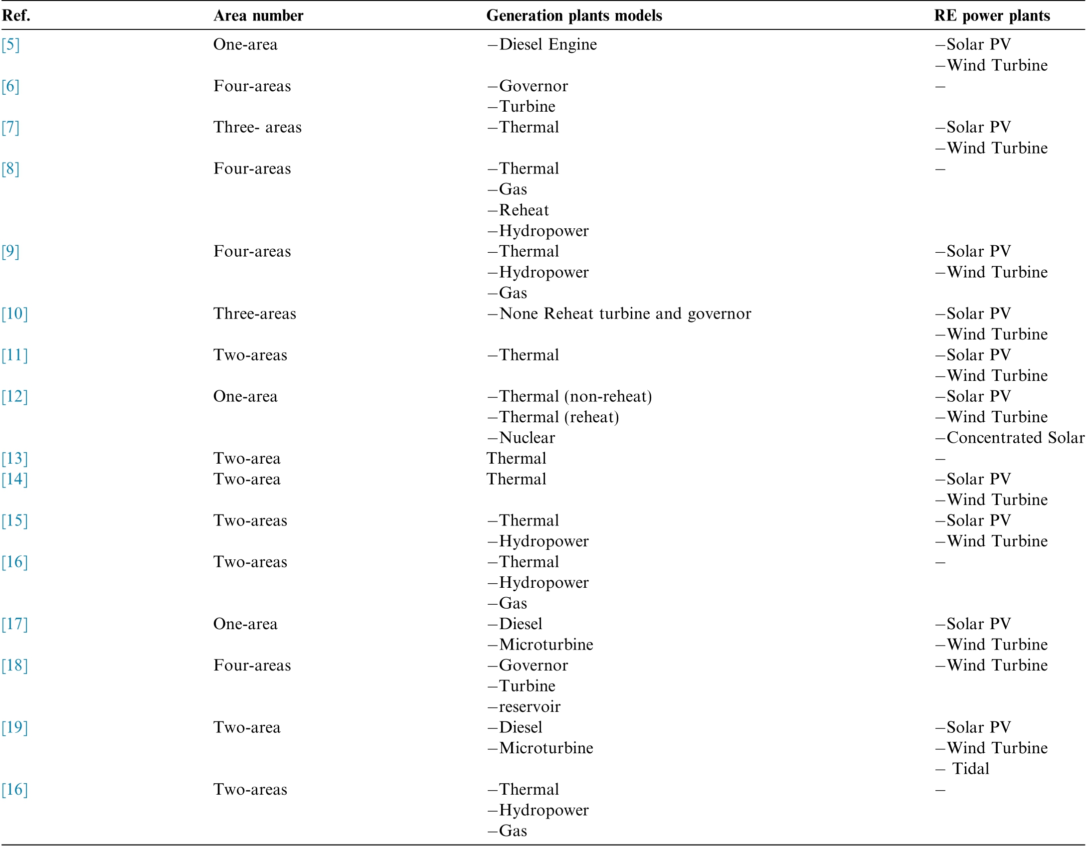
The paper will be divided into the following Sections1 modelling and methodology of the interconnected power system.Section 2 results and discussion include the testing scenarios and the power systems frequency responses.Section 3 Conclusion summarizes the results and highlights the important findings.

1 Modelling and methodology

1.1 System overview

The Malaysian peninsula grid consists of three distinct areas, each with its own generation mix. The North Region consists of thermal power plants, Gas, hydro,and Solar PV. Whereas the South Region is not equipped with any Solar PV plants,the East Region consists of both Solar PV plants and Hydropower plants. The unique mix of solar thermal, gas, and hydropower plants makes the grid essential to understand how contingencies propagate in the system. A more noticeable feature of the systemis the connections between each area. The North and South Regions are connected to two areas through an AC tie line,while the Central and East are connected to three other areas at the same time. Fig. 1 shows the connectionsof each region with other regions through the AC tie lines.

1.2 Power plant models

Modelling of the power system utilized the established transfer functions and the dynamic model of each power plant. The Thermal Power Plant (TPP) generates electricity by converting mechanical energy stored in gas to rotational energy by passing it through the steam governor.The steam governor turns the thermal turbine connected to the generator for electricity generation. To improve the efficiency of the process, reheat turbines are used to extract more energy from the previously used steam by increasing its tempe rature. The main components of the TPP can be modeled using transfer functions[20] as shown in Fig. 2. Tt grepresents the thermal governor time consta nt. Krt and Trtcoefficient of steam reheat turbine and re heat turbine time constant, respect ively. Tttrepresent the thermal turbine time constant.

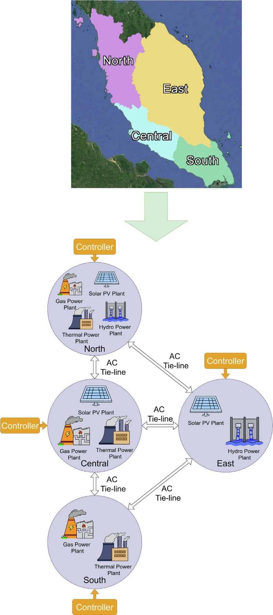
Fig. 1. Peninsular Malaysia grid overview.

Fig. 2. Thermal power plant model.

A Hydropower Plant (HPP) generates electricity from the stored potential energy in water. The hydro governor rotates when the valve allows water into the plant. The governor consequently turns the turbine to generate electricity. Transient droop compensation improves stability during transients by damping any undershoot or overshoot. All three major components of the HPP are modele d [20,21] as represented in Fig. 3.Thgrepresents the hy dro governor main servo. Tr and Trhrepresents the speed governor rest time and transient droop time consta nt, respectivel y. Twrepresents the water time constant.burning fuel. The valve position controls the amount of gas used for combustion and hence turns the gas governor.The fuel system models the combustion response of the plant. The compressor discharge system models air dynamics affecting the plants’ performance. The main components representing GPP [20,21] are shown in Fig. 4. b and arepresent the dynamic and static coeffi-cie nts, respectively. X and Yrepresent the governor lead and lag, respectivly. Tcr and Tfrepresent the combustion re action time delay and the fuel time constant, respectively. Tcdsrepresents the combustion reaction time delay.

A Gas Power Plant (GPP) generates electricity from is a basic transfer function model of conversio n of the Solar irradiance to PV power [22,23]. K pv and T pvrepresent the gain of the solar inverter and the inverter time constant, respectively. This model is leveraged over other models due to the simplicity in setting the solar power when studying different penetration levels.

To simulate the transfer function models, MATLAB/Si mulink is used for the simulation and testing of the

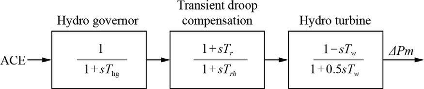
Fig. 3. Hydropower plant model.

Fig. 4. Gas power plant model.

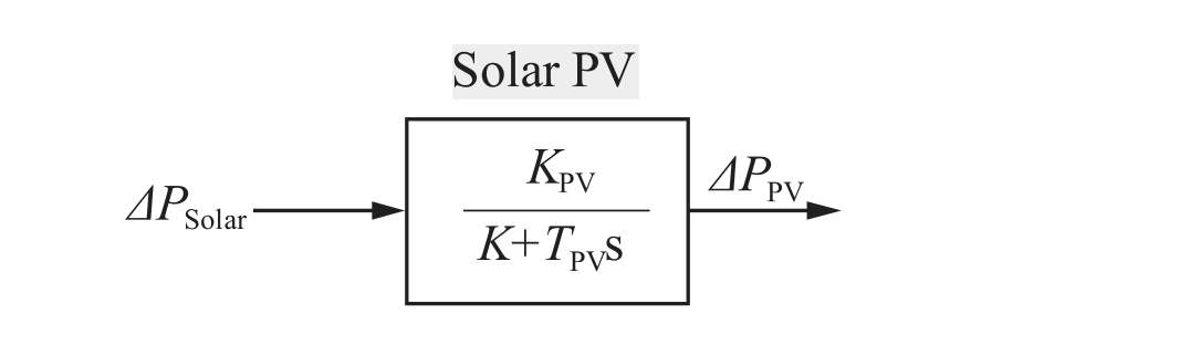
Fig. 5. Solar PV model.

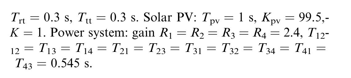
The Solar PV plant model is shown in Fig. 5. The model model. The complete dynami c interconnected modelis shown in Fig. 6 with the unique AC interconnection between regions and the power system and damping model. All the models and tie-lines Ttime constants are available in the appendix. The major contribution of this model is the mix of generation types in each region with varying inertia, additionally the unique AC interconnections between areas.

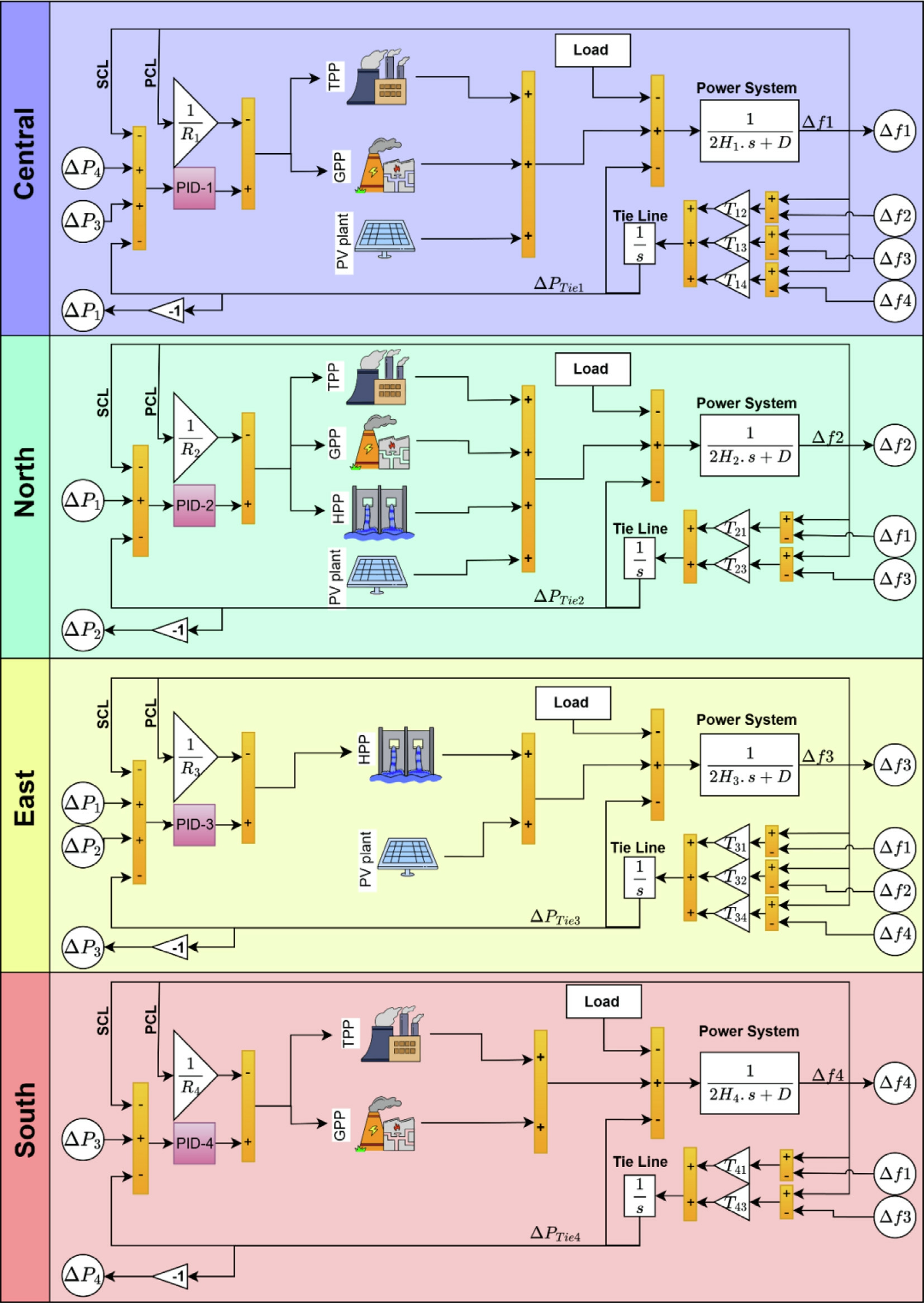
Fig. 6. Dynamic frequency control model.

1.3 Inertia estimation

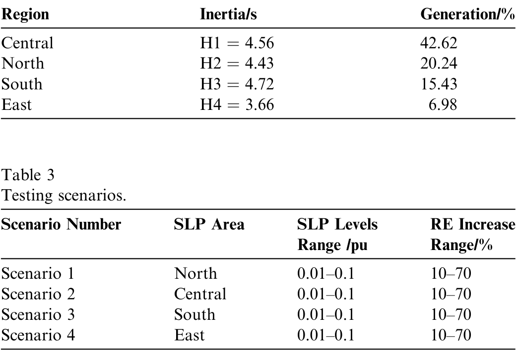
As demonstrated, the Malaysian power system has mixed types of generators. The generator’s inertia value varies based on generation type and on the capacity [24].As for the Solar PV, they are primarily inverter-based resources (IBR) and lack rotating parts, hence do not contribute to inertia. To estimate the inertia of each region,the rated power of each region was obtained,and the inertiaof each generator was estimated based on [24]. The inertia can then be calculated with (1), where Heqis the equivalent rotating mass inertia.

where is the inertia constant for i-p ower plant, and SB iis the rated power of the i - power plant. S B is the rated power ofthe power system, including IBR, and CGis the total number of conventional generat ors. Each region’s inertia was calculated independently from the other while accounting for Solar PV plants. The inertia and the percentage of generation of each region are listed in Table 2.

2 Results and discussion

The root of frequency fluctuation in the power system lies in the supply–demand imbalance. To evaluate the power grid, different scenarios were devised where a Step Load Perturbation (SLP) is applied with a range of 0.01 p.u. to 0.1 p.u. with 0.01 p.u. step. Malaysia’s plan toincrease the RE capacity to 70% by 2050 [2]. Consequently, in each scenario, Solar PV penetration level increased by 10% to 70% while adjusting the inertia contribution. Four Scenarios were devised with the SLP level ranges and RE Increase ranges, with the main difference being the location of SLP, as detailed in Table 3. SLPs are the focus of the study due to the type of imbalance they cause the system, whereas they force the frequency to be reduced significantly and hence produce a frequency nadir.

Table 2 Pe ninsular Malaysia grid inertia and generation.

2.1 Scenario 1: North region disturbance

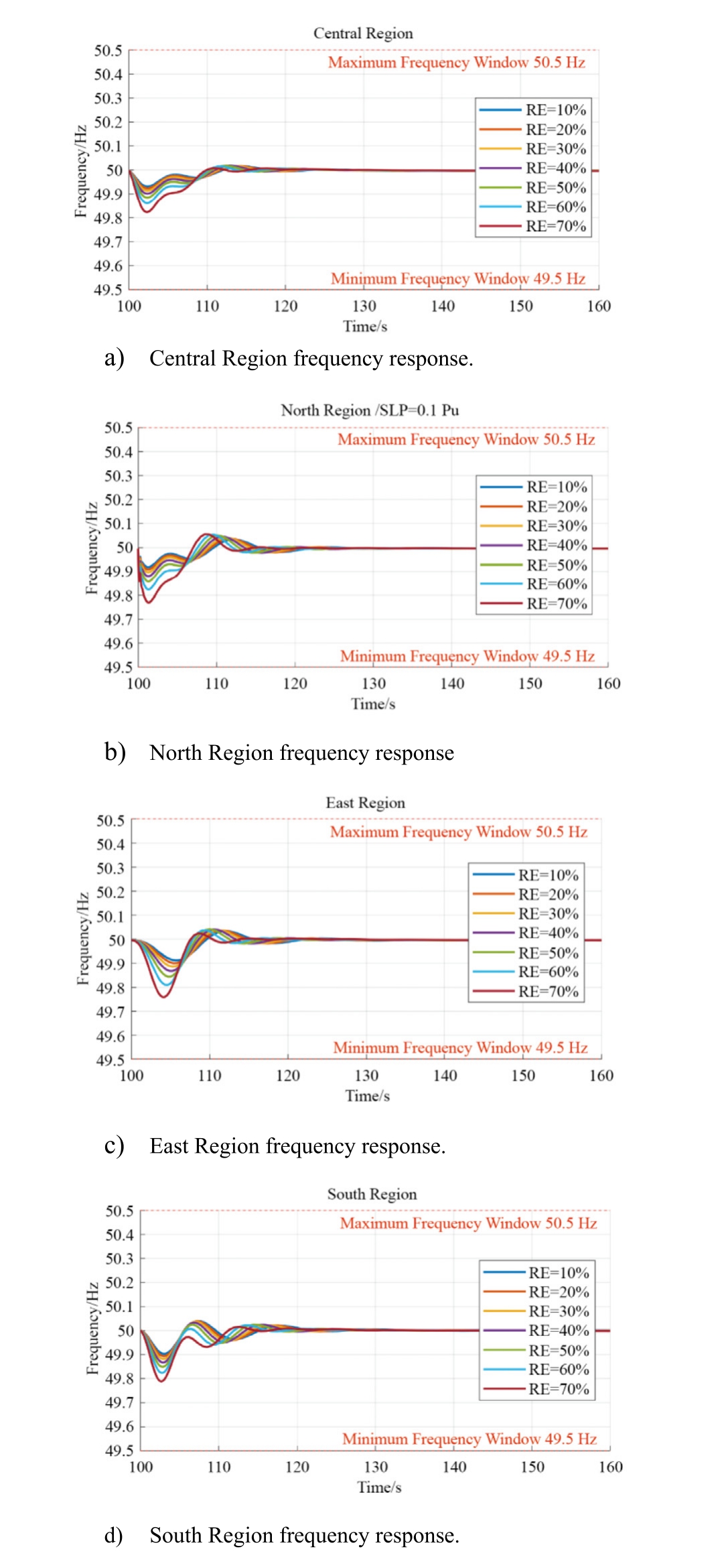
Fig. 7. Scenario 1 frequency response.

In this scenario, the SLP was applied in the North Region. First, the RE level was varied while fixing the SLP level to 0.1p.u.The frequency response of each region isshown in Fig. 7. Fig. 7b shows that the increase in load causes the frequency to drop before the generation starts to increase, and the system rest ores balance. The remaining parts of the network are Fig. 7 a, c and d, which show a similar frequency response. The system shows robustness even with the highest level of RE increase, where the frequency nadir does not surpass the limit set by Malaysia’s grid operator[24]. The increase in RE causes the frequency nadir to increase across the system. To measure the relation between the increased RE penetration, SLP level,and frequency, a new performance metric is proposed mFDand is shown in (2).

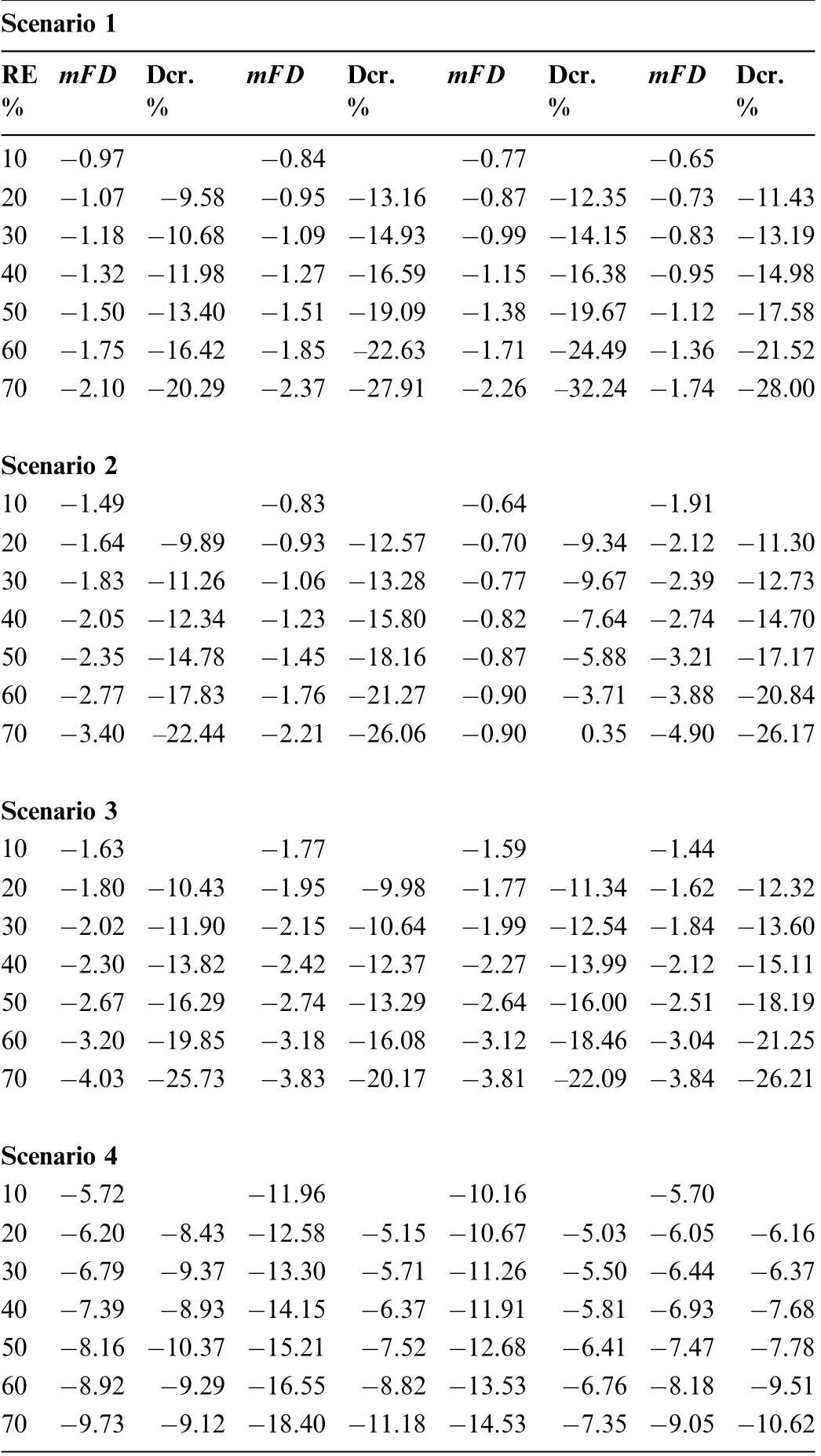
ΔF nadir is the change of frequency nadir.ΔD isturbance is the change of SLP level. F nadiri r is the frequency nadir at point i with a penetration percentage level of r.Di sturbancei r is the SLP level at point i with penetration percentage level of r.The metric shows the slope of t he change of frequency nadir corresponding to the change of SLP level at different RE levels. Stated differently, the sensitivity of the frequency nadir as the SLP changes.A deeper examination of the metric shows that an increased chang e in the frequency nadir causes the metric to increase, indicating an increased sensitivity. The opposite is correct when evaluating the change of disturbance.A poor frequency nadir can be a result of one of the following or a combination. A decrease in system inertia produces lower frequency nadirs. System damping affects mainly the oscillatory component of the frequency with limited effects on the frequency nadir [25]. Furthermore,a poor controller can affect the dynamic response of the system, triggering lower frequency nadirs. This metricis plotted with its corresponding RE penetration level increase to observe the change and is shown in Fig. 8.

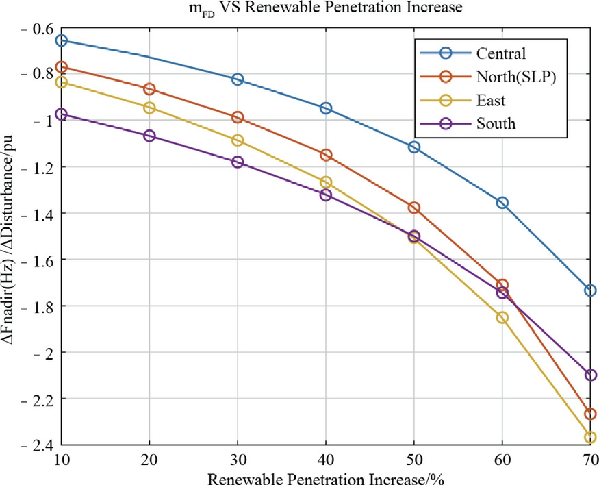
Fig. 8. Scenario 1 sensitivity of frequency nadir.

From Fig. 8, it can be observed that an increase in RE penetration level causes a decrease in mF D indicating increased sensitivity to increased SLP levels, in this scenario. The South region is the least affected region with the least sensitivity owing to the remoteness of the South Region when compared to the location of the SLP. The East shows the most sensitivity due to its reduced inertia when compared to other regions. The central area is the least affected due to its higher inertia despite its proximity to the SLP applied location.

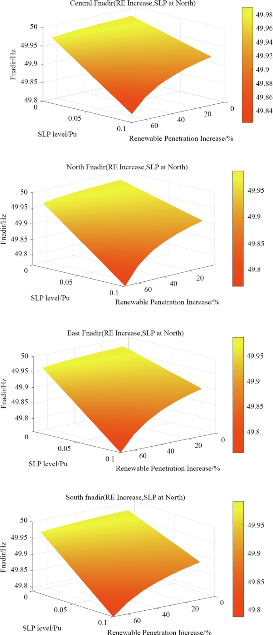
Fig. 9. Scenario 1 frequency nadir as function of SLP andRE penetration.

Fig. 9 shows the 3D graphs of the frequency nadir in different regions as a function of RE penetration level increase and SLP level increase. It shows a similar trend in all the regions.The increase in SLP level shows a linear increase in frequency nadir across all regions. This is attributed to the increase of imbalance of larger SLP produces in the system. However, RE increase causes the system to be more susceptible to an increase of frequency nadir even when SLP level is the same. Furthermore.The worst frequency nadir can be observed to be when the highest RE level is present with the highest SLP level.

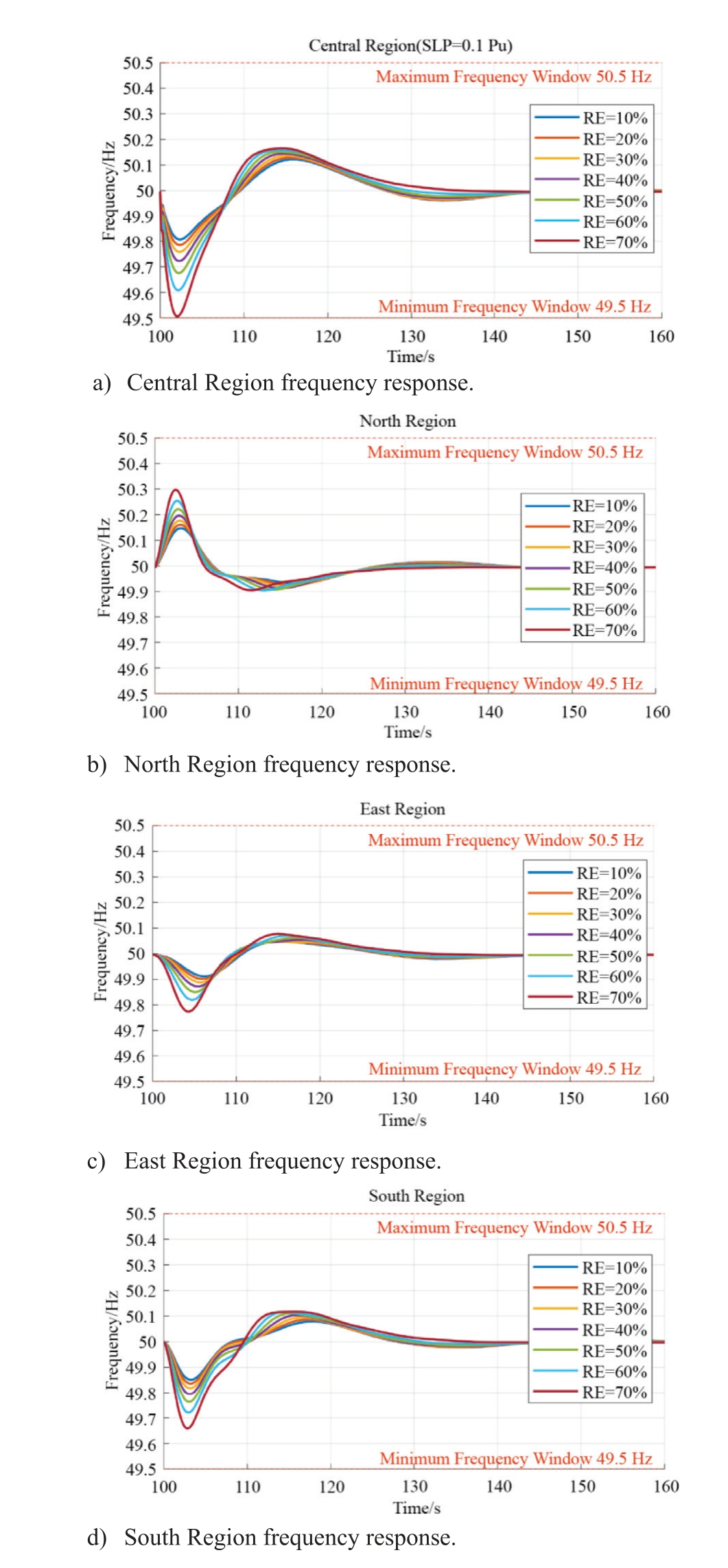
Fig. 10. Scenario 2 frequency response.

2.2 Scenario 2: Central region disturbance

Fig. 10 shows the performance of the system when the RE pentration level is increased to 70% with a 10% step whereas an SLP of 0.1 p.u. is applied in the Central Region.

Fig. 10a shows the system frequency nadir increases significantly as RE penetration increases. The lowest frequency nadir value recorded is 49.5 Hz, whereas it is on par with the lowest allowed frequency by the Malaysian grid operator [24]. The Central Region, shown in Fig. 10b shows an increase in frequency. This is attributed tothe generation mix, whereas in the North it generates 20.24% of the grid consumption compared to the central region with 42.62% generation. The increase in load at the central forces the system in the north to increase its generation to balance its regional frequency. Fig. 10c and d show the frequency in the East Region and South Region, respectively. The frequency in the East shows less frequency reduction than in the South. This is due to the East Region being connected to three other regions,assisting it in maintaining the supply–demand balance,whereas inthe South, it is connected to two regions, only one of which is under disturbance.etrationlevels.AstheNorth Regionfrequency overshot,

Fig.11showsthemFD ofthesystemat differentREpenthe frequency nadir was relatively stable at different RE penetration levels. The Central Region showed the most susceptibility to an increase in RE penetration, whereas itcarries the most generation percentage in the system,and reducing its inertia while increasing RE increases its sensitivity to disturbances compared to other regions.The East Region shows the best resilience to an increase indisturbance levels, with the increase of RE due to its interconnection to three regions, aiding in the system balance. Conversely, the South Region shows more susceptibility due to its connection to two regions,of which one is under SLP.

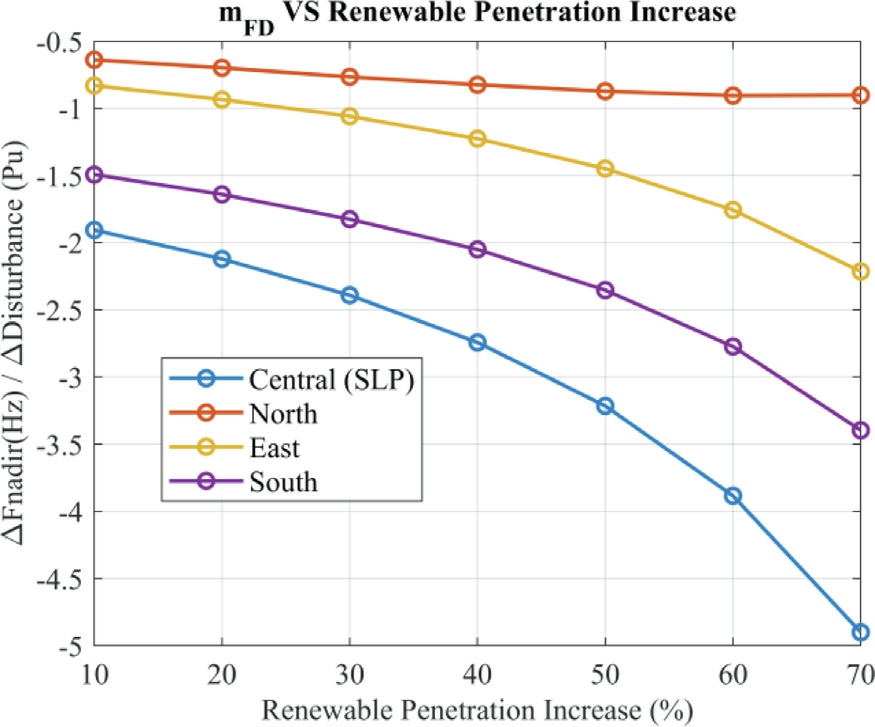
Fig. 11. Scenario 2 sensitivity of frequency nadir.

Fig. 1 2 shows the 3D graphs of the frequency nadir in different regions as a function of RE penetration level increase and SLP level increase. The Central Region shows the lowest frequency nadir when the highest SLPis applied, with the highest RE level due to the SLP being applied in that region. The North Region shows less susceptibility to changes in frequency nadir due to the overshoot behavior of the frequency. The South and East Region show similar behavior when the RE and SLP are increased. Furthermore, the linear relationship between SLP and Frequency nadir is still the same, and the relationship be tween RE power and frequency nadir is still the same as well.

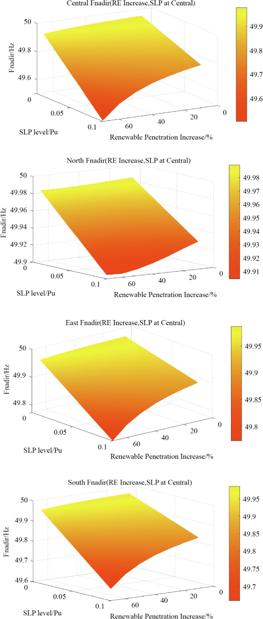
Fig. 12. Scenario 2 frequency nadir as function of SLP andRE penetration.

2.3 Scenario 3: South region disturbance

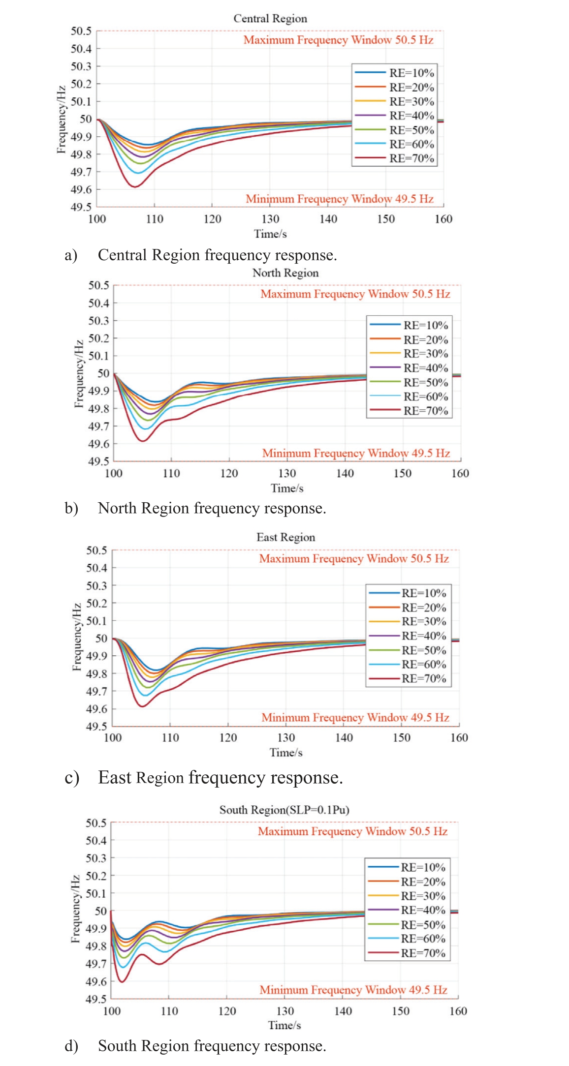
Fig. 13. Scenario 3 frequency response.

Fig. 13 shows the frequency response with varying RE and SLP of 0.1p.u. ap plied in the South Region. All the regions, Fig. 13a, b, and d, have a similar response with the frequency reducing post SLP application in the South Region. The increase of RE causes the frequency nadir to bethe lowest across all regions. However, a distinct difference that can be observed is how fast each region takes to hit the frequency nadir. The South Region, Fig. 13d,shows the sharpest reduction to frequency nadir. The slowest red uction to frequency nadir is in the Central Region,Fig. 13a, when compared to the East Region, Fig. 13c.This is attributed to the high inertia in the Central Region when compared to the East Region.

The frequency nadir sensitivity to disturbance at different RE, mFDof scenario 3 is shown in Fig. 14. The sensitivity is very closely aligned in all regions until the penetration level is 60%. The East Region has the worst sensitivity due to its lower inertia compared to the other systems. The North and South Regions have very closely aligned sensitivity. The Central Region is the best due to itshigh-power generation and high comparative inertia.When RE penetration is 60% and above, the trend changes, where the South Region becomes the most susceptible to reduced frequency nadir due to SLP being applied at that region, while the other regions approach the same sensitivity. The relatively same sensitivity at the penetration level is due to each region’s own characteristics. Whereas the Central Region has the highest generation and the most inertia. The North Region is far from the SLP location. The East Region is interconnected with three different regions, two of which are stable and resilient, giving aid in its resilience.

Graphs of the frequency nadir in different regions as a function of RE penetration level increase and SLP level increase are shown in Fig. 15. The relation in this scenario issimilar to the other, with the highest frequency nadir recorded across all regions when the RE and SLP are at their highest values. In this scenario, the relation of SLP and frequency nadir is similar in all regions is descending linearly,whereas higher SLP causes lower frequency nadir points.

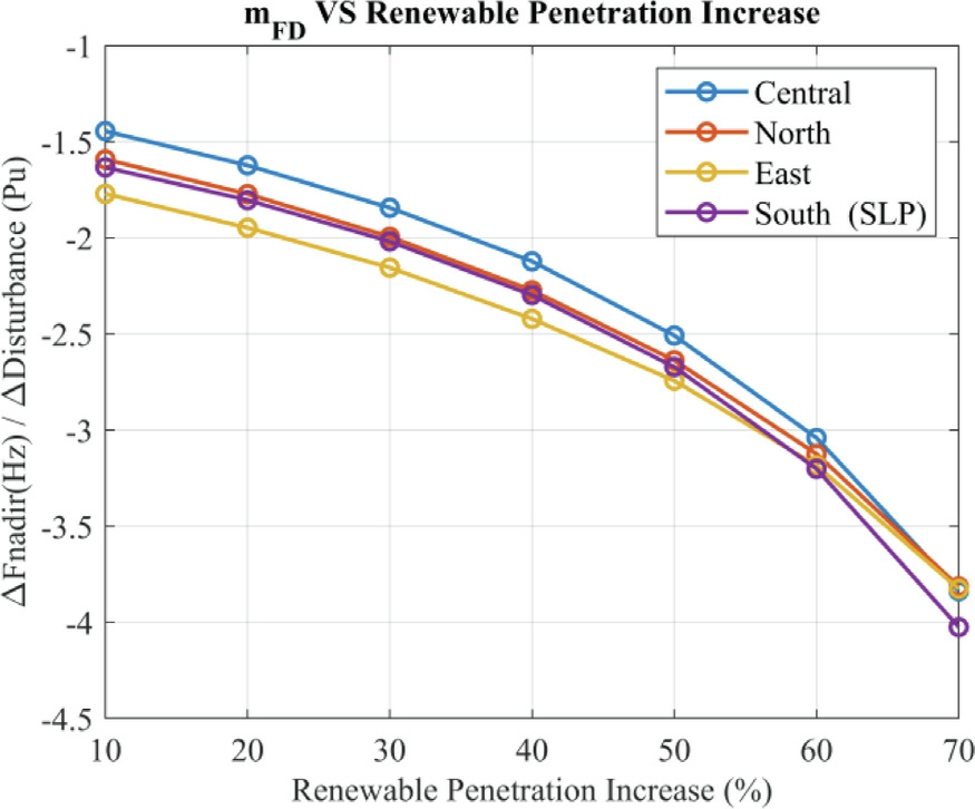
Fig. 14. Scenario 3 sensitivity of frequency nadir.

2.4 Scenario 4: East region disturbance

Fig. 16 shows the performance of the system when SLP isapplied in the East Region. The system’s general response behaviour in this scenario is similar to that of scenario two.sh

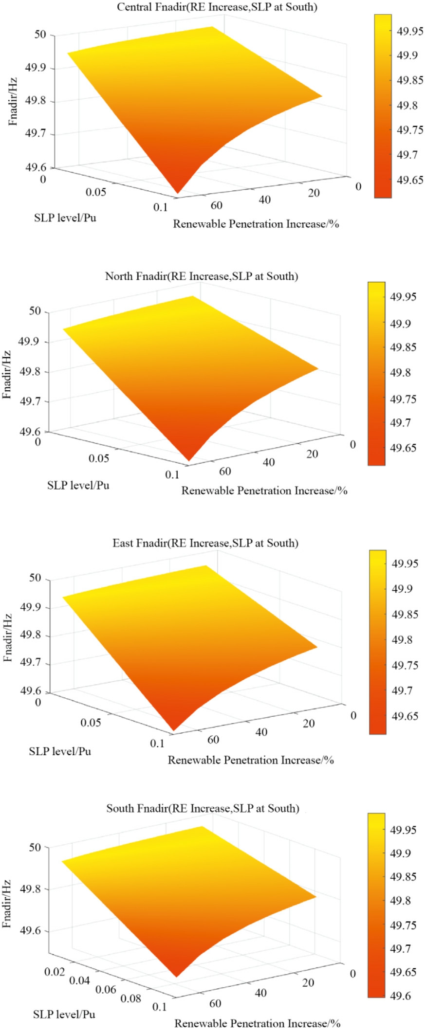
Fig. 15. Scenario 3 frequency nadir as function of SLP and RE penetration.

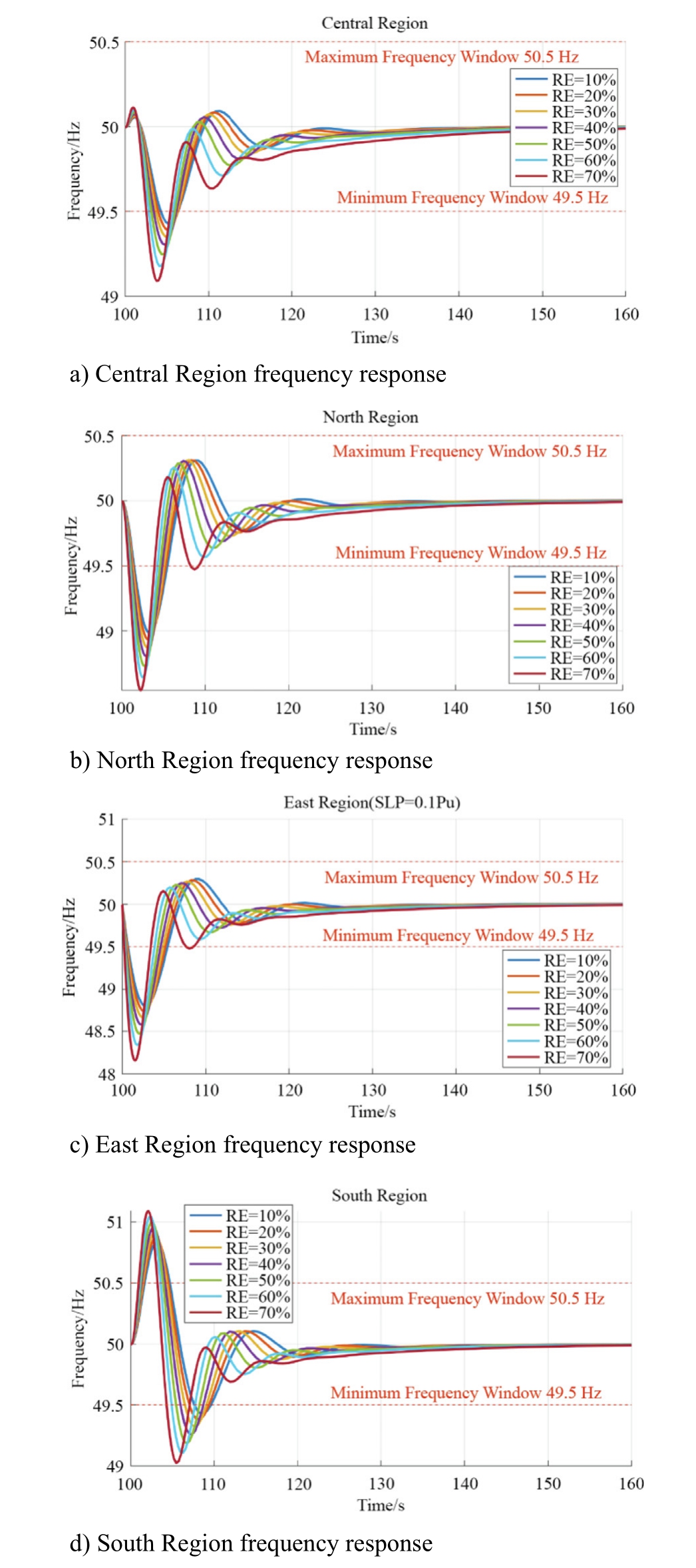
Fig. 16. Scenario 4 frequency response.

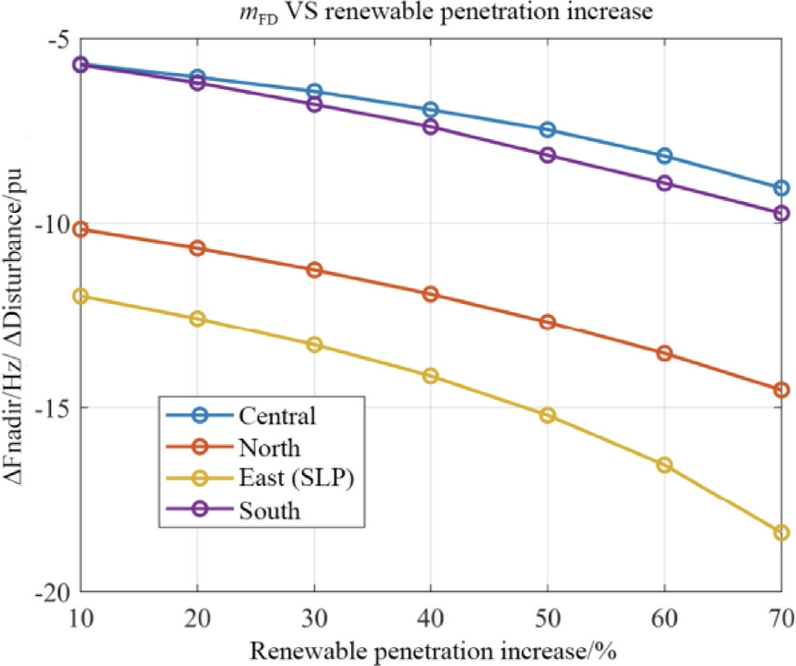
Fig. 17. Scenario 4 sensitivity of frequency nadir.

Nonetheless, the values of frequency nadir and overoot are very different.The East Region is the region with the least generation percentage, hence 0.1 p.u. is a large amount compared to its generation capability. As a result,the frequency nadir exceeds the allowable minimum window, as shown in Fig. 16c. The other regions get affected similarly. Fig. 16b shows the North Region with a lower frequency when compa red to the Central Region in Fig. 16a. The South Region shows an increase in generation, causing the frequency to overshoot. This is due to the South Region being the second least generation percentage after the East, and the South Region attempting to stabilize the power flow. Consequently, this is why there is a better frequency response in the Central Region when it is compared to the North Region, as it is connected directly to the South Region and due to it having higher inertia.

The frequency nadir sensitivity to disturbance at differ-

ent RE, mFD,of scenario 3 is shown in Fig. 17. The Centr al Region showed the most resilience to an increase in RE due to its high inertia in the system. The South Region follows, and then the North Region. The worst sensitivityis in the East Region due to its reduced inertia and the SLP being located at it.

Fig. 18 shows the 3D plot of the frequency nadir asa function of the change of RE penetration level and SLP.The general trend across all regions is relatively the same as scenario 2. However, this scenario shows significantly the worst frequency nadir and susceptibility to RE penetrations, with the worst frequency nadir recorded at the highest SLP and the highest RE level.Due to the low generation percentage in the East Region, where the SLPis applied, and hence hinders the stability of the rest of the system.

The operator needs to consider a higher generation reserve with inertia, alternatively, equipping the system with virtual inertia devices, to ensure the interconnected power system can maintain its stability.

3 Concl usion

Even though the results conclude similar behavior in all regions, key findings can be concluded from the model based on the Malaysian grid and how to anticipate the frequency behavior when accommodating a higher RE penetration level in the interconnected systems.

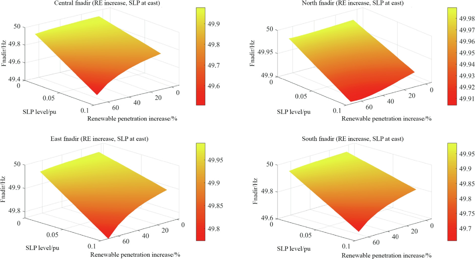
Fig. 18. Scenario 4 frequency nadir as function of SLP and RE penetration.

Inertia plays a major role in the stability of an interconnected power system. Reduced inertia in one region more than the others hinders the system stability and causes major issues across the other interconnected systems.

The increase in RE penetration levels causes the system tobe more sensitive to any disturbance with varying levels,asshownwith performancemetricsproposedmFD.Even if the disturbance islow in magnitude,theincrease inRE penetration and the consecutive reduction in inertia exposes the system to the worst frequency nadirs. However, this exposure is further limited in an interconnected system by each area’s inertia levels. The relations in the testing scenario show that more than 60% of the increase inRE penetration levels cause the system stability to deteriorate faster. This is due to the significant reduction in inertia equipped generation mix among the interconnected areas.

The location where a frequency contingency occurs can have varying effects across the system. An area with reduced inertia can cause cascading effects on the frequency fluctuation across the system. However, the opposite does not apply in higher inertia regions.Furthermore,the effects of contingency in a region with high inertia are much less on further away regions.

The interconnections of areas are both beneficial and detrimental to the system. More interconnections to a low inertia region help with its reliance only when the contingency is not in the same region. In contrast, the region can cause the most harm to the power system if a continge ncy were to happen in it.

The research shows how an interconnected system’s performance can vary significantly with different parameters of inertia, RE penetration levels, SLP Magnitudes and SLP location. The research aids in the best allocation ofsynthetic inertia devices as more IBR are being connected to the grid, whereas low inertia areas should be prioritized with synthetic inertia devices due to the suscept ibility they cause to the system if a contingency were to happen in it. Areas with higher penetration levels should be maintained with high inertia or replaced with synthetic inertia devices due to the role they play in mitigating the propagating effects of contingency from one region to another through them.

Based on these findings, actionable recommendations for the grid operator can be made. The East region is the most susceptible to the reduced inertia effects, and it’s recommended to equip the region with virtual inertia devices, such as energy storage systems, as the inertia is reduced in the system.Alternatively,the region could have ahigher reserve of controlled generation sources equipped with inertia.

Highlighting the limitations of the model, the power plants are assumed to have lumped up generators of the same kind, whereas the generators could have different parameters within the same area. Moreover, the tie line power capacity is constant among areas. Furthermore,the speed the plant can react to when disturbance occursis based on the inherent non-linearities of the plant and communication delays among areas and within the area itself.In addition, different categories of supply–demand imbalance can be examined in future research. The sufficient size of synthetic inertia devices in different regions needs tobe studied based on the control topology method. Additionally, verification of the nonlinear relationship of the performance metric and the RE penetration level canbe further evaluated against other interconnected power system models. These limitations can be addressed in future research to further understand the propagating effectsof disturbances in an interconnected system.

CRediT authorship contribution statement

Ousama M.T. Ajami: Writing – original draft, Visualization, Validation, Methodology, Formal analysis, Conceptualization. Maadh S.J. Alkhusaibi: Data curation,Investigation, Methodology, Software, Writing – review& editing. Rodney H.G. Tan: Writing – review & editing,Visualization, Validation, Supervision, Methodology,Funding acquisiti on, Conceptualization. Farah Adilah Jamaludin: Writing – review & editing, Supervision, Project administration, Funding acquisition. Mithulananthan Nadarajah: Writing – review & editing, Validation, Supervision, Resources, Project administration.

Declaration of competing interest

The authors declare that they have no known competing financial interests or personal relationshi ps that could have appeared to influence the work reported in this paper.

Acknowledgments

This work was supported and funded by the UCSI University Research Excellence and Innovation Grant[REIG-FETBE-2024/006].

Appendix A

Appendix B

References

[1]M. Denchak, Fossil fuels: the dirty facts, Nat. Res. Defense Council. (2022).

[2]Ministry of Economy, Malaysia, ‘‘National Energy Transition Roadmap (NETR).” Aug. 2023, [Online]. Available: https://www.ekonomi.gov.my.

[3]F. Chien, C.-C. Hsu, I. Ozturk, A. Sharif, M. Sadiq, The role of renewable energy and urbanization towards greenhouse gas emission in top Asian countries: evidence from advance panel estimations, Renew. Energy 186 (2022) 207–216, https://doi.org/10.1016/j.renene.2021.12.118.

[4]H.B. Tambunan, P.A.A. Pramana, B.S. Munir, Intermittent Renewable Energy Source (IRES) model of solar energy in Cipayung microgrid system, J. Phys. Conf. Ser. 1402 (3) (2019),https://doi.org/10.1088/1742-6596/1402/3/033103 033103.

[5]A.E. Khalil, T.A. Boghdady, M.H. Alham, D.K. Ibrahim,Enhancing the conventional controllers for load frequency control of isolated microgrids using proposed multi-objective formulation via artificial rabbits optimization algorithm, IEEE Access 11 (2023) 3472–3493, https://doi.org/10.1109/ACCESS.2023.3234043.

[6]I.A. Khan et al., Load frequency control using golden eagle optimization for multi-area power system connected through AC/HVDC transmission and supported with hybrid energy storage devices, IEEE Access 11 (2023) 44672–44695, https://doi.org/10.1109/ACCESS.2023.3272836.

[7]D. Boopathi, K. Jagatheesan, B. Anand, S. Samanta, N. Dey,Frequency regulation of interlinked microgrid system using mayfly algorithm-based PID controller,Sustainability 15(11)(2023)8829,https://doi.org/10.3390/su15118829.

[8]A.R. Sagor et al., Pelican optimization algorithm-based proportional–integral–derivative controller for superior frequency regulation in interconnected multi-area power generating system,Energies 17 (13) (2024) 3308, https://doi.org/10.3390/en17133308.

[9]T. Ali et al., Terminal voltage and load frequency control in a real four-area multi-source interconnected power system with nonlinearities via OOBO algorithm, IEEE Access 12 (2024)123782–123803, https://doi.org/10.1109/ACCESS.2024.3453755.

[10]M.M. Elsaied, W.H. Abdel Hameed, H.M. Hasanien, Frequency stabilization of a hybrid three-area power system equipped with energy storage units and renewable energy sources, IET Renew.Power Gener. 16 (15) (2022) 3267–3286, https://doi.org/10.1049/rpg2.12577.

[11]M. Amir, M. Zaery, K. Singh, S.M. Suhail Hussain, M.A. Abido,Enhancement of frequency regulation by TFOID controller in hybrid renewable energy with battery storage system-based multiarea microgrids, IEEE Access 12 (2024) 110813–110828, https://doi.org/10.1109/ACCESS.2024.3439738.

[12]M. Nour, G. Magdy, J.P. Chaves-á vila, á. Sánchez-Miralles, F.Jurado, A new two-stage controller design for frequency regulation oflow-inertia power system with virtual synchronous generator,J.Energy Storage 62 (2023), https://doi.org/10.1016/j.est.2023.106952 106952.

[13]Y. Zheng et al., Power system load frequency active disturbance rejection control via reinforcemen t learning-based memetic particle swarm optimization,IEEE Access 9(2021)116194–116206,https://doi.org/10.1109/ACCESS.2021.3099904.

[14]S. Ali et al., Frequency regulation in interconnected power system through enhanced beluga whale optimized flatness-based active disturbance rejection control,IEEE Access 12(2024)15348–15367,https://doi.org/10.1109/ACCESS.2024.3358425.

[15]A.M.A. Soliman, M. Bahaa Eldin, M. Ahmed Mehanna,Application of WOA tuned type-2 FLC for LFC of two area power system with RFB and solar park considering TCPS in interline, IEEE Access 10 (2022) 112007–112018, https://doi.org/10.1109/ACCESS.2022.3215530.

[16]M.F.A. Limon et al., Grey wolf optimization-based fuzzy-PID controller for load frequency control in multi-area power systems,J.Autom. Intell. (2025), https://doi.org/10.1016/j.jai.2025.01.002.

[17]A. Bouaddi, R. Rabeh, M. Ferfra, Load frequency control in autonomous microgrids using hybrid Algorithm GWO-CS based fuzzy logic sliding mode controller,Results Eng.25(2025),https://doi.org/10.1016/j.rineng.2025.104412 104412.

[18]H.H. Alhelou, N. Nagpal, N. Kassarwani, P. Siano, Decentralized optimized integral sliding mode-based load frequency control for interconnected multi-area power systems, IEEE Access 11 (2023)32296–32307, https://doi.org/10.1109/ACCESS.2023.3262790.

[19]P. Samal, N. Nayak, A. Satapathy, S.K. Bhuyan, Load frequency control in renewable based micro grid with Deep Neural Network based controller, Results Eng. 25 (2025), https://doi.org/10.1016/j.rineng.2024.103554 103554.

[20]Z.X. Tang, Y.S. Lim, S. Morris, J.L. Yi, P.F. Lyons, P.C. Taylor,Acomprehensive work package for energy storage systems as a means of frequency regulation with increased penetration of photovoltaic systems, Int. J. Electr. Power Energy Syst. 110(2019) 197–207, https://doi.org/10.1016/j.ijepes.2019.03.002.

[21]K.S. Ramakrishna, P. Sharma, T. Bhatti, Automatic generation control of interconnected power system with diverse sources of power generation, Int. J. Eng. Sci. Technol. 2 (5) (2010), https://doi.org/10.4314/ijest.v2i5.60102.

[22]P.A. Gbadega, A.K. Saha, Load frequency control of a two-area power system with a stand-alone microgrid based on adaptive model predictive control, IEEE J. Emerg. Sel. Top. Power Electron. 9 (6) (2021) 7253–7263, https://doi.org/10.1109/JESTPE.2020.3012659.

[23]J. Heidary, M. Gheisarnejad, H. Rastegar, M.H. Khooban, Survey onmicrogrids frequency regulation:modeling and control systems,Electr. Power Syst. Res. 213 (2022), https://doi.org/10.1016/j.epsr.2022.108719 108719.

[24]Energy Commission of Malaysia, ‘‘Grid Code for Peninsular Malaysia”. 2020.

[25]V. Cuvicins, A. Sauhats, and V. Strelkovs, ‘‘Problems of Frequency Control in the Power System with Massive Penetration of D istributed Generation”, 2008, [Online]. Available: https://api.semanticscholar.org/CorpusID:14047567.

Received 28 July 2025;revised 12 November 2025; accepted 20 November 2025

Peer review under the responsibility of Global Energy Interconnection Group Co. Ltd.

E-mail addresses: 1001748783@ucsiuniversity.edu.my (O.M.T.Ajami), 1002164737@ucsiuniversity.edu.my (M.S.J. Alkhusaibi ), rodneytan@ucsiuniversity.edu.my (R.H.G. Tan), farahadilah@ucsiuniversity.edu.my (F.A. Jamaludin), mithulan@eecs.uq.edu.au (M. Nadarajah).

https://doi.org/10.1016/j.gloei.2025.11.005

2096-5117/© 2026 Global Energy Interconnection Group Co. Ltd. Publishing services by Elsevier B.V. on behalf of KeAi Communications Co. Ltd.

This is an open access article under the CC BY-NC-ND license(http://creativecommons.org/licenses/by-nc-nd/4.0/).

Ousama M.T. Ajami completed his bachelor’s degree in electrical and Electronics Engineering with (hons.) from UCSI, Malaysia in 2023.Currently he is pursuing a Ph.D. at UCSI university, specializing in power system frequency sta bility using ESSs and control optimization.