0 Introduction

The construction of wind farms is justified by the need tomeet the growing energy demand in Brazil,reduce greenhouse gas emissions,and mitigate risks associated with the current Brazilian energy model by diversifying energy sources.According to data from the National System Operator (ONS),the installed wind energy capacity reached 20,655 average MW in 2022,increasing to 25,491 average MW by the end of 2023,representing an annual increase of 23%[1].This growth,particularly notable in the Northeast subsystem,is due to substantial investments,establishing Brazil as a global leader in wind energy generation.Wind energy generation is intrinsically linked to stochastic processes of meteorological variables,reflecting the random and unpredictable nature of these parameters.Stochasticity in the context of wind energy refers to the direct dependence on weather variables,which are inherently volatile and dynamic.

In this context of high variability and uncertainty,longterm forecasting emerges as a strategic tool to achieve objectives for both efficient wind farm operations and long-term planning in the renewable energy sector.The ability to anticipate the future generation curve over months or years allows companies to develop more efficient and financially profitable energy portfolio management strategies.Through this forecasting,it is possible to align energy production with more favorable market conditions,optimizing the trading of power purchase and sale agreements.By adjust ing the production curve to market opportunities,proftis can be maximized,ensuring that generated energy is sold during periods of higher demand and elevated prices.

From a strategic planning perspective,anticipating future generation and climatic behaviors enables the optimization of preventive and corrective maintenance schedules,ensuring turbines operate under ideal conditions during periods of expected high generation.Planned maintenance,supported by long-term forecasts,minimizes unplanned downtime,which could result in production and revenue losses.Furthermore,by avoiding unexpected failures that may require emergency corrective actions,operators reduce the risk of compromising operational effi-ciency and extend the lifespan of equipment,given that most decision-making and administrative processes in wind farms,such as budgeting,resource allocation,and maintenance scheduling,are conducted in monthly or quarterly cycles [2].

In the current context,marked by high availability of meteorological and operational data,data science,especially machine learning,emerges as a tool for predictive analysis of time series.These concepts apply algorithms and data mining techni ques,such as artificial neural networks,support vector regression,and decision trees,to extract patterns and insights from large data volumes.Additionally,data science enables the implementation of real-time monitoring systems,using streaming processing techniques to detect operational anomalies and optimize predictive maintenance of wind turbines.This approach increa ses efficiency and equipment lifespan,maximizing wind energy production and contributing to the reliability ofrenewable energy supply [3].

Within the spectrum of machine learning techniques,there are methods like Ridge Regression and Random Forest.Ridge regression is a variant of classical linear regression,introducing a regularization term that penalizes high coefficients,particularly in datasets where variables are highly correlated.On the other hand,Random Forests aggregate multiple independent decision trees,each built from random samples of the dataset and subsets of features,to capture complex nonlinear interactions and important variables that may be challenging to identify with linear models.

Moreover,techniques such as Support Vector Machines(SVM) and Multilayer Perceptron (MLP) Neural Networks are highly valued for their capabilities in classification and regression problems [4].Support Vector Regression (SVR) is known for its robustness in highdimensional spaces and its effectiveness in optimizing separation hyperplanes,leveraging kernel methods to handle non-linearly separable problems[5].MLPs consist of multiple layers of interconnected neurons,capable of modeling complex nonlinear relationships thanks to their hidden layers,distinguishing them from simple perceptron’s.The training of MLPs uses the backpropagation algorithm to adjust synaptic weights and minimize errors,enabling the network to generalize from data,achieving significant performance in tasks such as time series forecasting and pattern recognition [6].

Gradient Boosting,in turn,stands out for its effectiveness across a wide range of applications,positioning it as astate-of-the-art method for classification and regression.eXtreme Gradient Boosting (XGBoost) is an advanced and scalable implementation of this technique,recognized asa modern tool in data science research.A key factor of XGBoost is its scalability,supporting faster operations than conventional methods on individual machines and being scalable to handle billions of examples in distributed ormemory-constrained environments [7].

This article addresses the principles of modeling strategies,drawing on state-of-the-art advancements in machine learning techniques and their application in renewable energy generation forecasting.The research demonstrates that these techniques contribute to optimizing energy production,enhancing the efficiency and profitability of wind farms.The general structure of the study is shown in Fig.1.

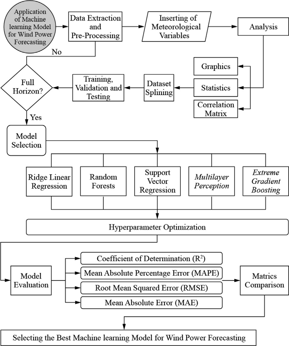
Fig.1.Global structure of the methodology of the study.

1 Background

The complementarity of machine learning models must be fundamentally tied to climatic variables and meteorological context,as the effectiveness of these models depends on the correct integration of atmospheric phenomena with wind energy generation patterns.Understanding concepts related to wind dynamics is essential to capture the complex interaction between weather conditions—such as variations in wind speed,wind direction,and other climatic factors—and the response of wind turbines.The volatility and predictability of winds,crucial elements for wind turbine performance,are theoretically addressed,exploring turbine design characteristics and energy efficiency.

In the case of the Pindaí Wind Complex,used as a case study for the application of machine learning methodologies,these aspects become even more relevant.Located in the municipality of Pindaí,in the south of the stateof Bahia,the Pindaí wind co mplex has an installed capacity of 79.9 MW,divided into four distinct wind farms: Pindaí I with 16.45 MW,PindaíII with 18.8 MW,PindaíIII with 21.15 MW and Pindaí IV with 25.5 MW,illustrated in Fig.2.

Fig.2.Pindaí wind complex.

The wind turbines of the complex were built by Wobben Windpower/ENERCON,specifically of the Enercon E-92 model.The turbines have a nominal powerof 2,350.0 kW,with their power curve presented in Fig.6.Notably,in the wind speed range between 1 and 25 m/s,the turbine starts operating in a transient state until reaching 50% of its total generation capacit y.During this phase,the azimuth (blade/rotor orientation) is continuously adjusted until the blades become perpendicular to the incoming wind.Each turbine has a diameter of 92.0m and a height of 98.0m,with aswept areaof6,648.0 m2,maximizing wind capture.The turbines feature three blades,optimizing kinetic energy conversion and ensuring mechanical stability.The turbine hub can be adjusted between a minimum height of 85 m and a maximum height of 138 m,allowing flexible operation to adapt to different wind conditions.Meanwhile,the blade tip speed can reach up to 77 m/s,enhancing energy generation efficiency while maintaining structural integrity and compliance with safety standards.

The complex is subject to various atmospheric systems that affect both synoptic and mesoscale wind regimes,directly impacting operational efficiency.Analyzing the diurnal,seasonal,and interannual variability of wind,with emphasis on phenomena such as El Niño and La Niña,is crucial to understanding fluctuations in wind patterns and their influen ce on energy generation.Understanding this atmospheric variability allows for the optimization of the complex’s operation and management,guiding the selection of techniques and parameters in generation forecasting models,and ensuring more efficient utilizationof wind energy in the region.

The operational definition used by the United States National Oceanic and Atmospheric Administration(NOAA) characterizes El Niño conditions as Sea Surface Temperatures (SSTs) in the central tropical Pacific that are 0.5°C warmer than average,while La Niña conditions are defined as SSTs 0.5°C cooler than average.These conditions must persist for five consecutive seasons to constitute a complete ENSO episode.During El Niño events,the warming of Pacific Ocean waters leads to a reconfiguration of atmospheric circulation patterns,often resulting in reduced rainfall and higher temperatures in northeastern Brazil,including Bahia.The phenomenon tends to exacerbate drought conditions,affecting water resources and agriculture,increasing wind energy production while reducing hydroelectric generation due to changes in wind regimes.On the other hand,La Niña events,characterized bycooler-than-average sea surface temperatures in the Pacific,are generally associated with increased rainfall and lower temperatures in northeastern Brazil.These conditions reduce wind energy production potential by influencing wind patterns,while also favoring agricultural conditions due to increased water availability.

1.1 High resolution weather forecast reanalysis models

In this study,meteorological variables derived from reanalysis models are used,encompassing both historical and forecasted data,adapted to the specific horizon related tothe Pindaí Wind Complex,such as air temperature,relative humidity,precipitation,surface pressure,wind speed at10 m,wind speed at 100 m,and wind gusts.These modelsare designed to capture atmospheric dynamics at different scales,ranging from broad weather systems to localized phenomena such as storms or microclimates.They are developed by international meteorological services,such as the Deutscher Wetterdienst (DWD) in Germany,NOAA in the United States,Météo-France in France,among others.Data extraction is performed through an API in JSON format provided on the Open-Meteo platform using open-source tools[8].An algorithm written in Python language enables querying the chosen exogen ous variables and setting search parameters.

Data extraction begins using the latitude and longitude coordinates of the gridpoint where the Pindaí complexis located,at latitude 14°29′ 24′′ South(-14.5) and longitude 42°41′ 24′′ West (-42.5).The date rangeforquerying historical variables is from July 1,2014,to December 31,2022.The variables are provided on an hourly basis and subsequently aggregated to a monthly basis.

For all parameters,a combination of meteorological models called Best Match was established,gathering information from the European Centre for Medium-Range Weather Forecasts (ECMWF),ERA5 (ECMWF Reanalysisv5 -the fifth generation of ECMWF atmospheric reanalysis with a spatial resolution of 31 km and a temporal resolution of one hour),ERA5 Land (reanalysis focused solely on land variables with a spatial resolution of 9 km),ERA5 Seamlessly (satellite data and surface observations with atmospheric and oceanic models),and CERRA(Copernicus Regional Reanalysis for Europe).For the forecasting stage,it will be necessary to update the time series with projections of met eorological variables from January 1,2023,to December 31,2023.Unlike historical variables,the forecasting system from Open-Meteo’s JSON API provides predictions based on daily rather than hourly data.

1.2 Machine learning

The algorithms considered in this paper were developed us ing Pyt hon and its libraries such as Scikit-Learn,TensorFlow,Keras,and Skforecast.Different machine learning techniques are explored,including ridge regression,random forests,support vector regression,mult ilayer perceptron,and eXtreme Gradient Boosting.Each model isoptimized with hyperparameters to enhance performance.

Seasonality and temporal dependencies in wind power generation data are intrinsically linked to atmospheric patterns and meteorological cycles,such as diurnal variations,synoptic-scale pressure systems,and seasonal wind regimes.In this study,these temporal structures were addressed implicitly through the design of the input feature set and explicitly through the modeling capabilities of the selected algorithms.Historical lag features (e.g.,generation values from previous days or months),moving averages,and time-based indicators (such as month or season) were incorporated into the training datasets to expose the models to recurrent patterns over time.Machine learning algorithms like XGBoost and Random Forest are particularly effective in capturing such patterns due to their ensemble-based structure,which can model non-linear relationships and conditional interactions between features.Meanwhile,algorithms like Support Vector Regression and Multilayer Perceptron can learn complex temporal dependencies when properly tuned and provided with temporally-encoded features.

1.2.1 Ridge regression

Ridge regression,a form of Tikhonov regularization,addresses instability in linear regression caused by multicollinearity.By modifying the least squares objective function with a penalty term proportional to the square of the coefficients,ridge regression balances the bias-variance tradeoff,mitigating overfitting.Introduced by Hoerl and Kennard [9],this technique incorporates a regularization parameter controlling the penalty magnitude,improving predictive performance and model interpretability.The coefficients are estimated by minimizing a cost function that includes this penalty.The equation for estimating the coefficients,considering the statistical criterion used,is described by the Moore-Penrose pseudoinverse formula(1):

where I is the identity matrix,Xis the design matrix (or feature matrix),y is the vector of observed responses,and αis the regularization parameter that controls the magnitude of the penalty applied to the coefficients [10].

Ridge regression imposes an L2 penalty on the regression coefficients,promoting stable solutions in the presence of multicollinearity,making it highly effective in problems where predictor variables are strongly correlated.Its methodological strength lies in analytical solvability and statistical robustness under Gaussian assumptions,yielding smoothed coefficients that tend to generalize well in high-dimensional,low-sample-size regimes.However,the assumption of linearity limits its applicability to problems involving complex interactions or nonlinearities,and the regularization-induced bias can hinder predictive accuracy if the penalty parameter is not optimally calibrated.

1.2.2 Random forest

Random Forests originated from the co ncept of decision trees and bagging.Breiman’s paper[11]laid the foundation by proposing an ensemble of decision trees built individually using bootstrap samples (a statistical resampling technique that involves random sampling with replacement) of the data and random subsets of features at each split.This approach addresses the high variance and underfitting tendencies of individual decision trees,improving prediction accuracy by aggregating multiple trees.The theoretical basis of Random Forests is rooted in the law of large numbers,where the ensemble’s prediction error decreases as the number of trees increases,provided the trees are uncorrelated.

The core of this technique lies in building a large number of decision trees during training and outputting either the mode of the classes (in classification) or the average prediction (in regression) of the individual trees.Randomness is introduced in two ways: through bootstrapping the data and through selecting a random subset of features for splitting at each node,ensuring diversity among the trees in the ensemble.This methodology is detailed in the work of Hastie,Tibshirani,and Friedman [12],emphasizing the balance Random Forests strike between bias and variance reduction and highlighting their effecti veness across a wide range of datasets and problem settings.

Their primary advantage lies in robustness to noise and outliers,with an innate ability to capture nonlinear interactions without requiring manual feature engineering.They also provide internal measures of variable importance and sample proximity,aiding exploratory analysis.However,their performance tends to deteriorate when extrapolating beyond the observed domain,and their black-box nature complicates formal interpretability.Furthermore,they can exhibit bias when handling categorical variables with many levels or under severe class imbalance.

1.2.3 Support vector regression

The concept of Support Vector Machines (SVM) has its roots in the 1960s.The basic idea of SVM,which involves the linear separation of data in a feature space usinga hyperplane,was introduced by Vladimir Vapnik and Alexey Chervonenkis in the Soviet Union in the early 1960s[13].However,it was in the 1990s that the technique gained prominence and became widely disseminated,especially after the introduction of non-linear kernels.These kernels allowed SVMs to be applied to non-linear problems by mapping the data into a high-dimensional space where a linear separation could be found [14].

Cortes and Vapnik’s 1995 paper[15]laid the foundation for the practical application of SVM,detailing the useof hyperplanes to separate data points in a highdimensional space.This was followed by extensive research on optimization algorithms used to solve the SVM problem,such as the Sequential Minimal Optimization (SMO) algorithm proposed by Platt [16]in 1998,which improved the co mputational efficiency of SVM.

At the core of the support vector machine approachis the concept of finding a hyperplane that best separates data points from different classes.The hyperplaneis defined by a subset of the training data known as support vectors,which are the critical elements that influence the hyperpla ne’s position and orientation.The algorithm can be formulated as an optimization problem,where the objective is to find a hyperplane or regression function that fits the data so that most points are within a specified margin of tolerance [15].The optimization problem canbe expressed by the formula (2):

where w is the weight vector,the hyperparameter C controls the penalty for deviations,εis the tolerance margi n,and are the slack variables that allow some predi ctions to be outside the tolerance margin.

Support Vector Regression (SVR) was designed to handle regression problems,extending SVM’s capability to predict continuous values instead of discrete labels.The basic approach of SVR involves creating a hyperplaneor regression function that minimizes prediction error while maintaining model simplicity through a penalty based on the norm of the coefficients [14].

SVR operates using a specific loss function called the epsilon-insensitive loss function,which ignores errors smaller than a given epsilon value.This feature allows SVR to focus on larger deviations while disregarding small variations,resulting in a model that is robust to data noise[5].Additionally,SVR uses support vectors,which are the data points outside the epsilon range,to define the regression function.This ensures that the model is determined only by the most critical data points,reducing the riskof overfitting [17].

SVR is distinguished by its convex optimization formulation,which guarantees global optima,and by its useof the ε-insensitive loss,offering precise control over model complexity and robustness to moderate noise.Leveraging the kernel trick,SVR operates in high-dimensional feature spaces implicitly,enabling accurate modeling of complex nonlinear relationships.However,its computational cost scales quadratically with the number of training samples,limiting scalability.Moreover,selecting the appropriate kernel function and tuning hyperparameters (such asC and γ) can be non-trivial,often requiring intensive crossvalidation and deep domain expertise.

1.2.4 Multilayer perceptron

The Multilayer Perceptron (MLP) is a class of feedforward neural networks (FFNN).An MLP consists of at least three layers of nodes: an input layer,one or more hidden layer s,and an output layer.The MLP differs from the single-layer perceptron in its ability to solve non-linear problems.The origins of MLPs trace back to the 1940s with the work of McCulloch and Pitts [18],who proposed acomputational model for neural networks based on algorithms and thresholds.The backpropagation techni que in multilayer neural networks was proposed by Werbos in 1974 [19].Backpropagation is an optimization algorithm that uses the gradient descent method to minimize the cost function of a neural network.The core idea of the algorithm is to compute the gradient of the error concerning the network weigh ts,propagating this error from the output layer back to the previous layers.This allows the weights to be iteratively adjusted to minimize the overall error of the network [19].

An MLP consists of several layers of nodes,each connected to the next layer.Each node,or neuron,in the network applies a weighted sum of its inputs and transmits the result through a non-linear activation function.Haykin discusses the importance of non-linear activation functions in the hidden layers of the MLP,such as the sigmoid and hyperbolic tangent function s.These functions introduce the necessary non-linearity for the MLP to model and learn complex relationships in the data,overcoming the limitation of the single-layer perceptron,which can only solve linearly separable problems.The choice of activation function can affect the network’s ability to model complex relationships [20].

Training an MLP involves adjusting the weights of the synaptic connections to minimize the error between the network’s predictions and the actual values of the training data.This process is primarily driven by the backpropagation algorithm,which computes the gradient of the loss function with respect to each weight in the network [21].The algorithm,along with an optimization method such asgradient descent,iteratively adjusts the weights in the direction that reduces the error,enabling the network to learn from the data [20].

Regularization techniques are used in multilayer neural networks to prevent over fitting,improve model generalization,and ensure the model performs well on new data.L2 regularization,also known as weight decay,adds a penalty proportional to the square of the weights’ magnitudes to the loss function[22].This encourages the network to keep the weights small,improving generalization by reducing model complexity.

Their primary technical advantage is architectural flexibility,especially when trained on large datasets,where they can learn hierarchical representations of the input space.Nevertheless,MLPs require meticulous tuning of hyperparameters and architecture,are sensitive to feature scaling,and prone to overfitting without explicit regularization or dropout.Moreover,their unstructured nature complicates interpretability and can lead to training instability.

1.2.5 Extreme gradient boosting

ExeXtreme Gradient Boosting (XGBoost) has established itself as an efficient machine learning method for a range of predictive tasks,due to its performance on structured data and its effectiveness in time series forecasting.Originating from the need for high-performance gradient boosting implementations,its origins can be traced back toFriedman’s introduction of Gradient Boosting Machines (GBM) in [23],which focused on minimizing a differentiable loss function for predictive learning problems.The journey from GBM to XGBoost involved a series of refinements aimed at improving speed and performance.Friedman’s stochastic gradient boosting [23],which introduced randomization into the fitting process to improve convergence rates and predictive accuracy,laid the foundation for these future improvements.XGBoost built on these advancements by form alizing a more regularized model to control overfitting,offering better performance.This introduction was made by Chen and Guestrin [7],defining it as a scalable system for gradient boosting capable of handling millions of instances beyond the scope of other algorithms at the time.

The eXtreme Gradient Boosting algorithm [7]is based ondecision trees,using the gradient boosting framework.This technique is part of the ensemble classifiers spectrum,which combines multiple predictive models to enh ance accuracy compared to individual models,based on the premise that weak models can be combined to form a strong model.

Among ensemble learning algorithms,the two main methods are called bagging and boosting.Boosting operates on the premise of sequentially improving ensemble performance by focusing on cases misclassified by previous models.This technique involves training a sequence of simple sub-models,with each subsequent sub-model adjusting its focus based on the errors of its predecessors.The aggregation of these sub-models results in a strong ensemble model with reduced bias and variance.The mathematics of boosting is embedded in its objective function,which seeks to minimize exponential loss,offering insight into the error correction mechanism of the algorithm [24].

In this framework,decision trees serve as the building blocks (sub-models),with each tree composed of nodes and branches.Tree construction begins with a single root node and proceeds by partitioning into subsets based on selected input variables.Partitioning continues until a stopping criterion is met,resulting in final predictions called leaves [24].Mathematically [7],given a dataset D with n observations and inputs of dimension m,the goal is to split D into subset s DLandDR that minimize a loss function L.

Splitting criteria determine how data is partitionedat each node to find the best split based on optimizing the loss function.For regression problems,the loss function is typically the mean squared error (MSE),defined by expression (3):

where y i are the actual values and ^yi are the predicted values.The gain G of a split at node j determines the best variable and split threshold and can be calculated by formula(4):

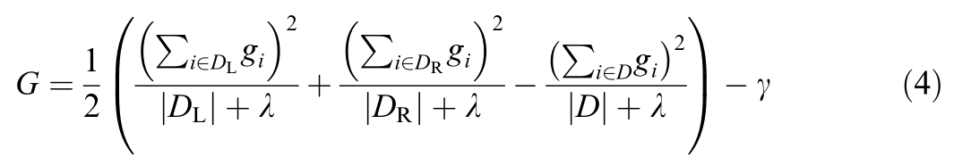
where is the gradient of the loss function concer ning the prediction ,λ is the regularization parameter co ntrolling complexity,and γ is the minimum loss reduction needed to make a split.Each summation represents the gradient sums for splits of observations DL,DR a nd D,respectively.

Regularization techniques introduce penalties to the loss function,discouraging overly complex models and promoting generalization.XGBoost uses two main forms of regularization,L1 (Lasso) and L2 (Ridge).These techniques are applied to the leaf weights of the decision trees,which are the values predicted by the leaves.The goal is to constrain these weights to low values,reducing model sensitivity to variations in the training data.

The performance of XGBoost is heavily dependent on hyperparameter tuning,which controls various aspects of model behavior.Hyperparameter optimization involves selecting the best set of parameters that maximize model predictive accuracy while minimizing over fitting and computational cost.

Boosting parameters influence the overall boosting process,including the learning rate,which determines the step size at each iteration,and the number of estimators,which defines the total number of trees in the model.Regularization parameters include the L1 and L2 terms discussed earlier.

The goal of hyperparameter tuning is to minimize the objective function,which comprises two components: the training loss and the regularization term [7].Mathematically,this is presented in expression (5):

where θre presents the hyperparameter space,L(θ)is the training loss (quantifying the model’s prediction error on the training data),and Ωdenotes the regularization term(penalizing model complexity to mitigate overfitting).

Its core advantage lies in its built-in regularization(both L1 and L2),which mitigates overfitting even in high-dimensional settings.Additionally,its native handling of missing values and level-wise parallelized tree construction contribute to superior performance compared to classical boosting techniques.However,the algorithm’s complexity hinders direct interpretability,and its performance can degrade in highly noisy datasets or when modeling higher-order,non-additive interactions—scenarios where neural networks often outperform.

2 Methodology

2.1 Data preprocessing

The historical generation data for the wind complex were collected over a 10-year time scale,from July 2014 to December 2023,in accordance with Fig.3.The raw time series was gathered on an hourly basis,totaling 228,000 observations,with 57,000 h for each wind farm.After data processing and normalization,using a transformation toa monthly basis,the time series for each wind farm was converted to 114 months of data.

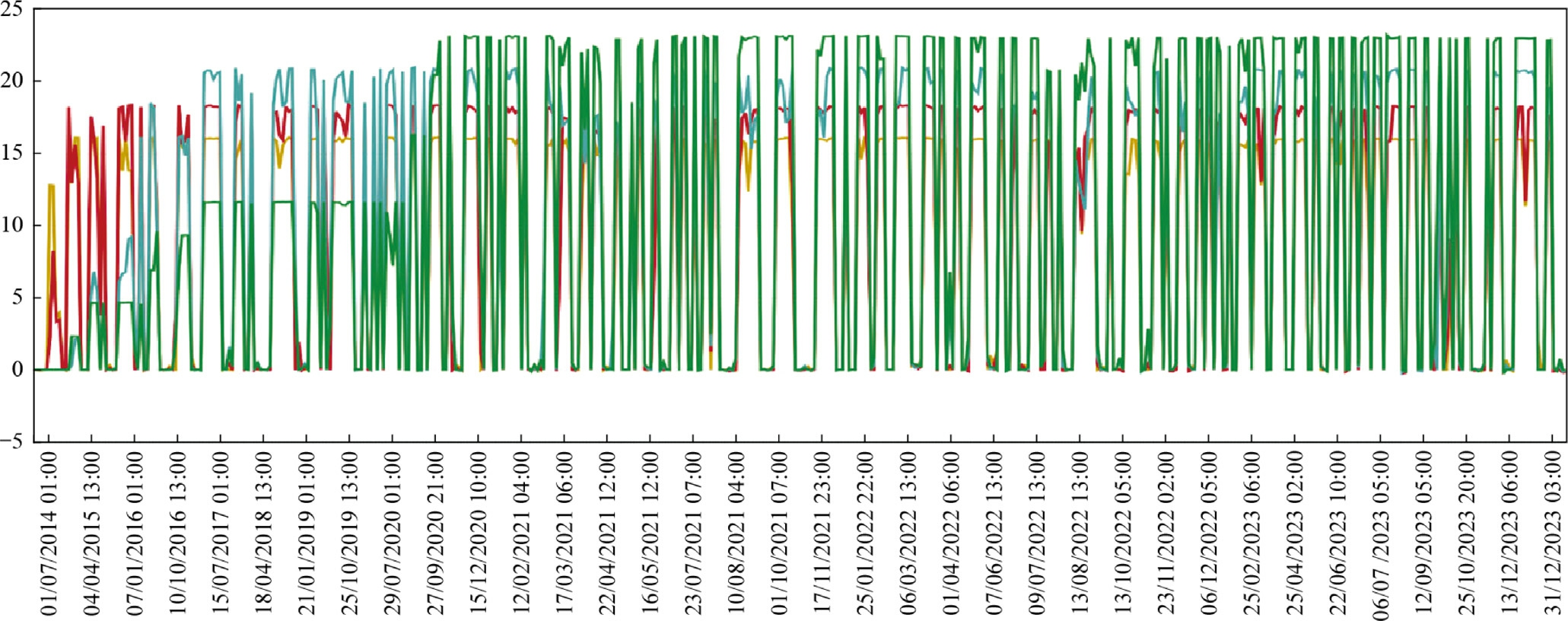
Fig.3.Historical generation data for the wind complex,from July 2014 to December 2023.

Hourly wind generation data contain a significant amount of detail,capturing,for example,fluctuations caused by meteorological changes over very short periods.With more than 80,000 h over nearly ten years,this discretization introduces a large degree of volatility and noise into the dataset.This can reflect vastly different conditions depending on the time of day,weather patterns,and local geographical influences,complicating the pattern recognition process.

Data extracted from storage systems often contain erroneous values due to various measurement issues.Faultyor poorly calibrated sensors can record incorrect values for power generation,wind speed,and other metrics.Given these measurement issues,it is crucial to perform a preprocessing step before aggregating hourly data intoa monthly-based time series.This step involves checking for missing or null data,iden tifying,and handling missing values that may occur due to sensor failures or data transmission interruptions.For this study,the Missing Completely at Random (MCAR) technique was applied.For missing hourly data,the average of the last 10 equivalent hours from previous days was used,along with the removal of duplicate data.

Fig.4 highlights the seasonal patterns that influence wind energy generation,which are intrinsically linked to climatic variations throughout the year.During the wet period,which extends from November to April,thereis a significant increase in precipitation,a phenomenon associated with the southward shift of the South Atlantic Convergence Zone.

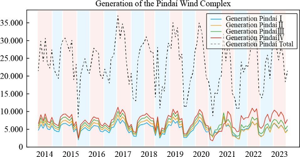
Fig.4.Highlights the seasonal patterns.

This shift causes a change in atmospheric conditions,resulting in decreased wind speeds in the region.This correlation is evidenced by the blue shading in the graph,which marks the months of higher precipitation.The reduction in wind intensity during this period contributes tolower turbine efficiency,consequently reflecting in lower energy generation levels.

In contrast,the dry period,occurring from May to October,is characterized by the northward retreat of the Convergence Zone,which substantially alters the wind regime.During these months,highlighted in red on the graph,there is a significant increase in wind speeds,favoring the operation of wind turbines.This seasonal change resul ts in higher efficiency in converting wind energy into electrical energy,increasing generation levels during this period.Such seasonal behavior is extremely relevant for the planning and optimization of wind farm operations,asit allows for the anticipation of energy production variations based on climatic patterns.

The boxplot graphs display the historical distribution of wind farm generation,revealing seasonal trends and energy produ ction variability aligned with regional climate patterns in northeastern Brazil.As discussed in Section 2.2 onthe climatological conditions of the Bahia region,wind generation seasonality is clearly divided between the wet period,from November to April,and the dry period,from May to October.This pattern is driven by regional meteorological conditions influenced by the Intertropical Convergence Zone (ITCZ) and local topographic features.

Figs.5–8 represent the boxplots of the historical generation distribution from 2014 to 2023 in MWh for the four mentioned wind farms.

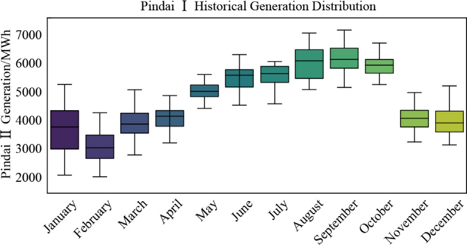
Fig.5.Pindaí I -Boxplot of the historical generation distribution from 2014 to 2023 in MWh.

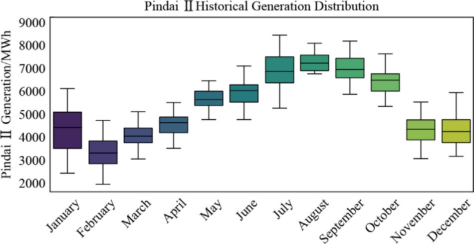
Fig.6.Pindaí II-Boxplot of the historical generation distribution from 2014 to 2023 in MWh.

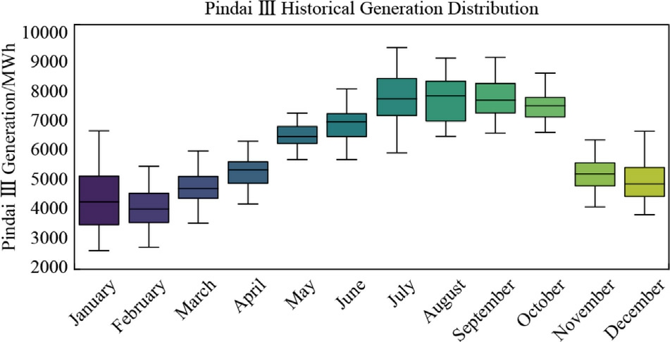
Fig.7.Pindaí III-Boxplot of the historical generation distribution from 2014 to 2023 in MWh.

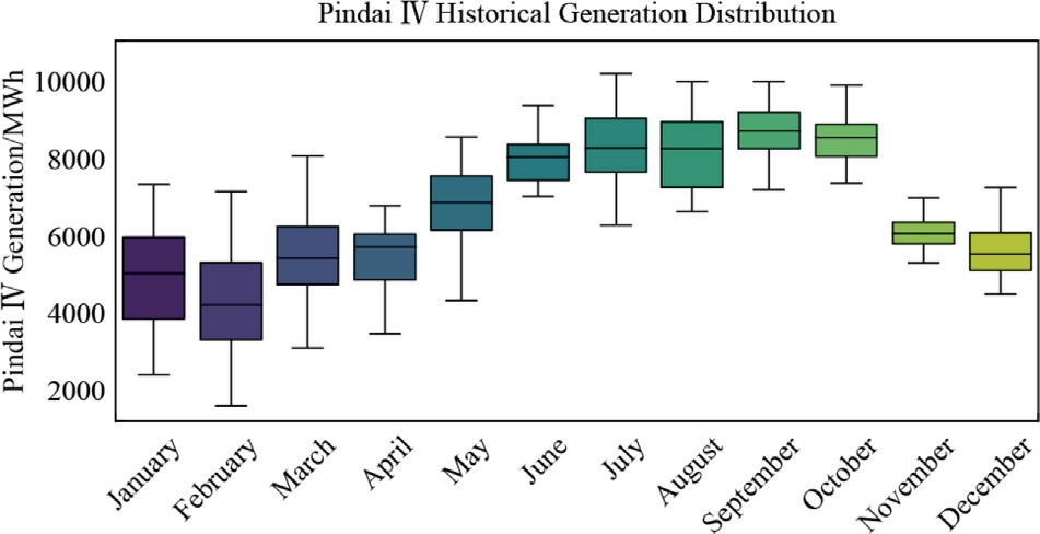
Fig.8.Pindaí IV-Boxplot of the historical generation distribution from 2014 to 2023 in MWh.

For Pindaí I Wind Farm,the data indicate a gradual increase in median wind generation from May to October,peaking during the dry season from July to August,with a median generation of 6000 MWh in the third quarter.In contrast,below-average performance is observed from November to April,characteristic of the humid climatic conditions of northeastern Brazil that prevail in the first half of the year.

Similarly,Pindaí II and III Wind Farms show even more pronounced seasonal fluctuations.For instance,Pindaí II starts with an average generation of 4900 MWh in January,escalating to a peak of 6900 MWh in August.The boxplot for PindaíIII reveals a considerable increase in both the median and the range of generation between June and August,with the median rising from 7000 MWh in June to 7900 MWh in August.

Pindaí IV exhibits the most abrupt changes,with average generation values rising sharply to 8400 MWh in August,accompanied by an expansion in the range of values,especially in the upper quartile.Across all wind farms,the lower quartile values gradually increase during the dry season.This indicates that even on days with relatively low wind speeds,energy generation does not drop as much asit does during the rainy season.In other words,during the dry season,even the least favorable days for wind energy generation still produce more energy compared to similar days in the rainy season.This seasonal impact is confirmed by the decline in generation from November to March,coinciding with the rainy season when wind speeds are generally lower and more inconsistent.

The correlation between generation and wi nd speedat 100 m can be seen in the scatter plots in Figs.9–12.Each point represents an observed pair of values: wind speedat 100 m and corresponding power generation.The distribution of points captures variability and trends within the data,while the regression line illustrates the average effect of wind speed on generation across the observed range.The positive slope of the line corroborates the previously quantified strong positive correlation with greater kinetic energy available in faster moving air masses,which turbines more efficiently convert into electrical energy.

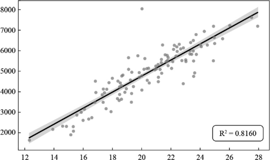
Fig.9.Pindaí I– Dispersion between historical generation and wind speed at 100 m.

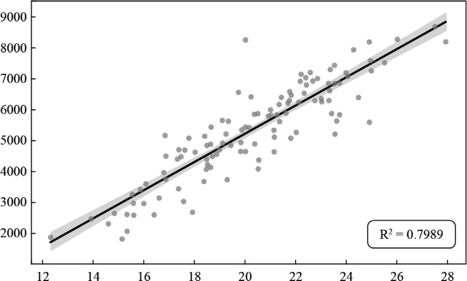
Fig.10.Pindaí II -Dispersion between historical generation and wind speed at 100 m.

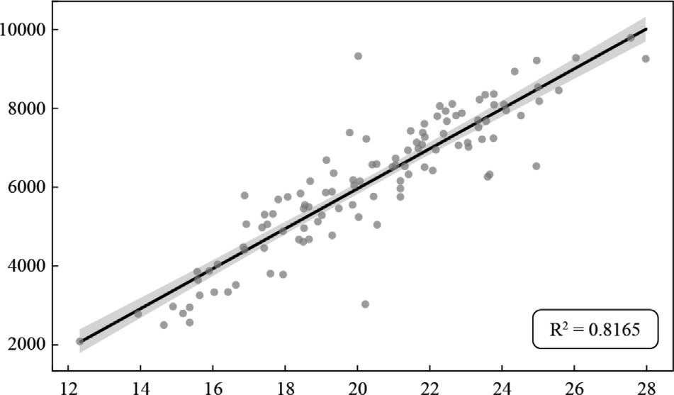
Fig.11.Pindaí III -Dispersion between historical generation and wind speed at 100 m.

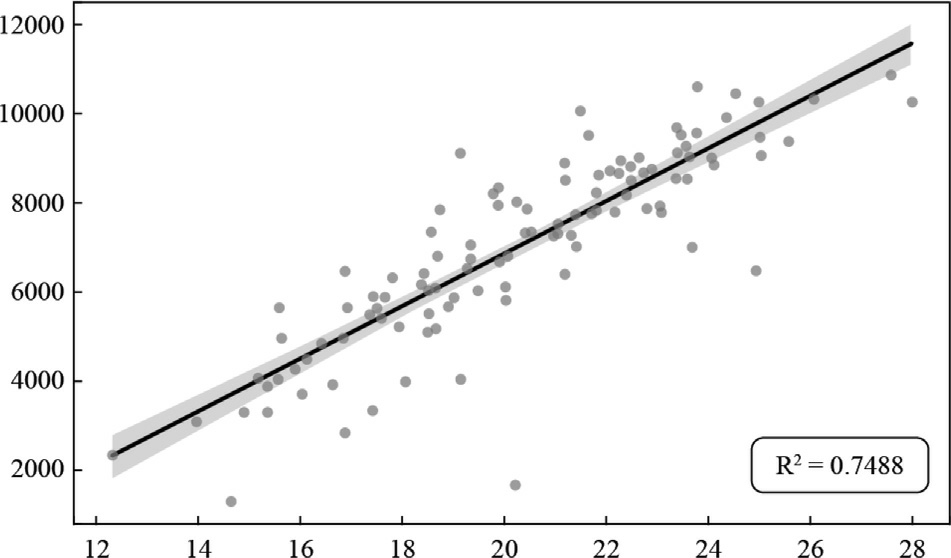
Fig.12.Pindaí IV -Dispersion between historical generation and wind speed at 100 m.

2.2 Parameter setting and implementation

Ridge Regression is implemented using the respective class from the Scikit-Learn library [25].Cross-validation tested 1440 different hyperparameter combinations (for each wind farm),according to the data in Table 1.The best choice for each hyperparameter is discussed as follows.

Table 1 Cross-validation tested for different hyperpa rameter combinations -Ridge Regression.

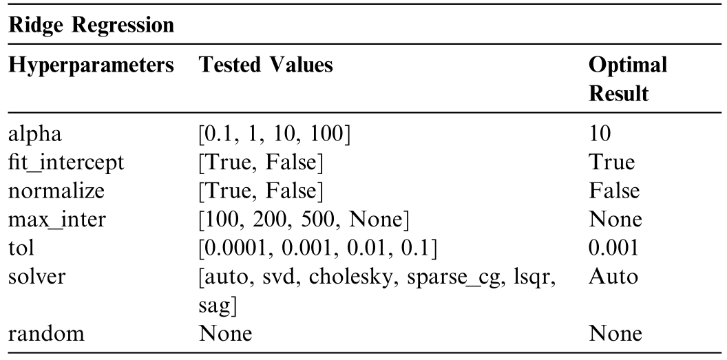
The optimization process incorporates the regularization parameter (alpha) set to 10.0,to enhance the conditioning of the problem and mitigate the variance of the parameter estimates.The fit_intercept parameter,set to True,specifies the inclusion of a constant term (biasor intercept) in the decision function.The normalize parameter is set to False,which,when combined with fit_intercept,ensures that input features are normalized prior to regression by centering them (subtracting the mean) and scaling them to unit norm.

The maximum number of iterations,max_iter,is set to None,indicating that the conjugate gradient optimization method will proceed without a predefined upper limit on the number of iterations.The precision of the solutionis controlled by the tol parameter,which is set to 0.001,defining the tolerance threshold for convergence.The solver parameter is set to auto,enabling the algorithm to dynamically select the most appropriate computational routine based on the dataset characteristics.Finally,the random_state parameter is set to None,leaving the random number generator seed undefined.While this parameter would typically influence reproducibility,it is applicable only if the selected solver differs from auto.

Regression with Random Forest is implemented using the related class from the Scikit-Learn library [25].Cross-validation,using the GridSearchCV class from Scikit-Learn,tested 186,624 different hyperparameter combinations (for each wind farm),as presented in Table 2.The best choice for each hyperparameter is discussed as follows.

Table 2 Cross-validation tested for different hyperparameter combinations -Random Forest.

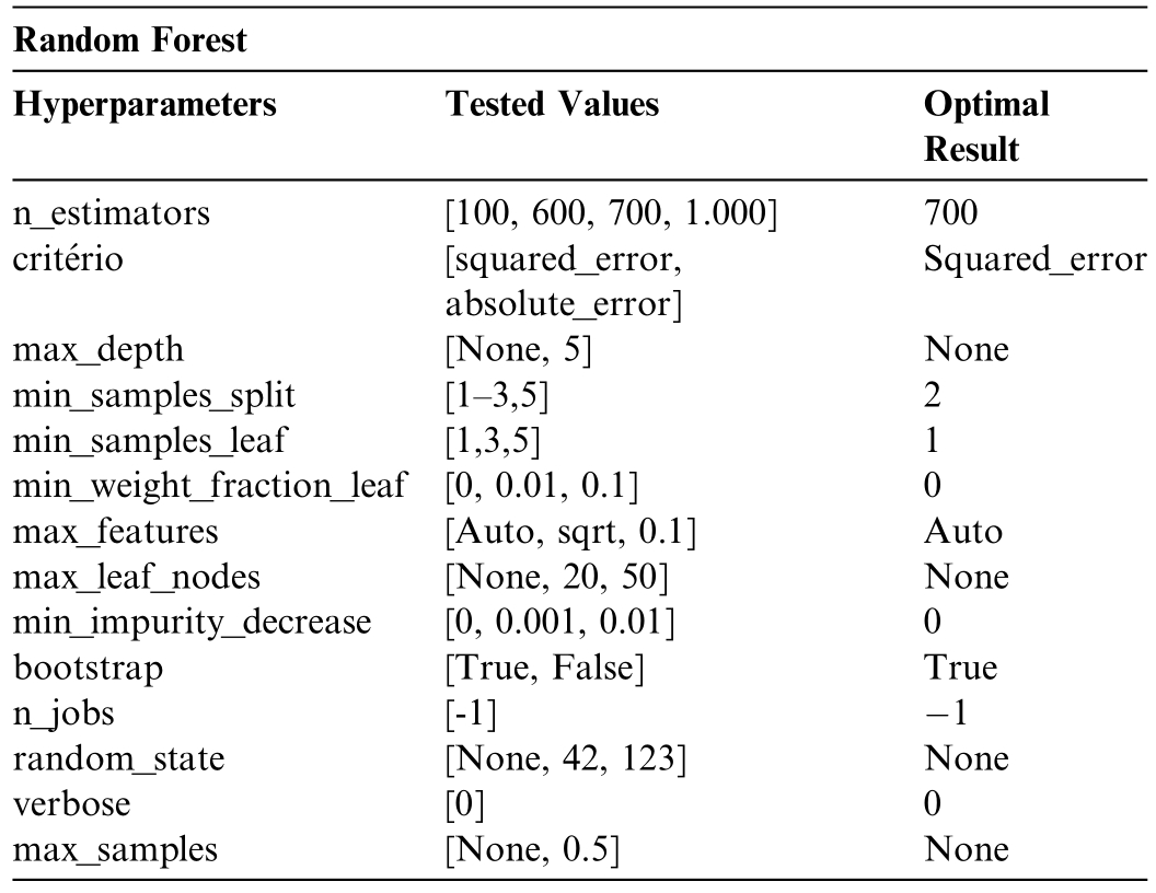
The parameter n_estimators,representing the number oftrees in the forest,is set to 100,establishing the ensemble size.The optimization criterion,criterion,is configured assquared_error,which evaluates the quality of splits by minimizing the mean squared error(MSE).The maximum depth of each tree,max_depth,is set to None,allowing trees to expand fully until all leaves are either pure or contain fewer samples than the minimum threshold.

The parameter min_samples_split,which specifies the minimum number of samples required to split an internal node,is set to 2.Similarly,the min_samples_leaf parameter,defining the minimum number of samples required to bepresent in a leaf node,is set to 1.The min_weight_fraction_leaf parameter,which ensures that a leaf contains at least a specified fraction of the total sample weights,is set to 0,disabling this constraint.The parameter max_features,indicating the number of features to consider when determining the best split,is set to auto,enabling the algorithm to automatically select the optimal subset of features.

The parameter max_leaf_nodes,which defines the maximum number of leaf nodes in each tree,is set to None,permitting unrestricted growth.The min_impurity_decrease parameter,control ling the splitting of nodes based onthe reduction in impurity,is set to 0,meaning no minimum threshold is enforced.

The bootstrap parameter,specifying whether sampling with replacement is employed during the construction of trees,is set to True.For parallel computation,n_jobs is set to -1,utilizing all available processor cores to maximize computational efficiency.The random_state parameter is set to None,meaning the randomness of the bootstrap sampling and feature selection process is not explicitly co ntrolled,which may affect reproducibility.The verbose parameter,governing the verbosity of logging output,is set to 0,suppressing detailed progress information.Finally,the max_samples parameter,determining the maximum number of samples drawn for training each tree,is set to None,ensuring that all available training samples are used.

Support Vector Regression was implemented using the SVR class from the Scikit-Learn library [25].Crossvalidation using the GridSearchCV class from Scikit-Learn tested 35,000 different hyperparameter combinations (for each wind farm),as shown in Table 3.The best choice for each hyperparameter is discussed as follows.

Table 3 Cross-validation tested for different hyperparam eter combinations–Support Vector Regression.

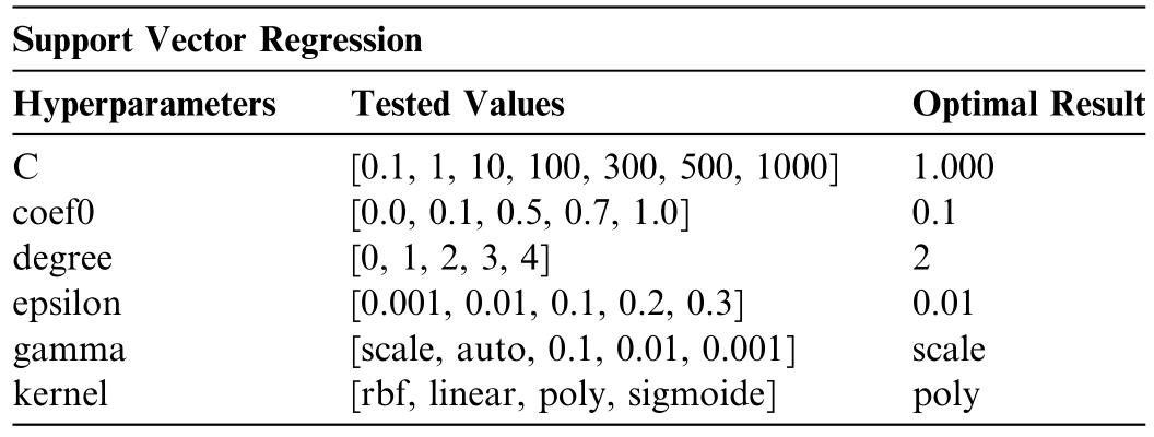
The hyperparameter C is set to 1000,controlling the regularization strength by penalizing errors.This parameter balances the trade-off between achieving a smooth decision boundary and accurately predicting training examples.The parameter coef0,an independent coefficient applied in polynomial and sigmoid kernels,is set to 0.1,influencing the shape of the decision bounda ry when these kernels are used.

The degree parameter,specifying the degree of the polynomial kernel,is set to 2,ind icating the use of a secondorder polynomial kernel for transforming the input feature space.The epsilon parameter is configured as 0.01,defining the width of the insensitive region in the loss function where deviations from the true target are not penalized,commonly used in regression tasks.

The gamm a parameter is set to scale,allo wing the algorithm to com pute its value automatically based on the dataset chara cteristics.This setting adjusts the influence of individual training points by scaling γ,which ensures adaptabi lity to different feature spaces.

The kernel function is specified as poly,de noting the use of a polynomial kernel.Additionally,the shrinking parameter is enabled (True),activating a heuristic that reduces the size of the optimization problem during training,thereby accelerating the convergence of the model.

Regression with a Multilayer Perceptron was implemented using the Scikit-Learn library[25]and TensorFlow Keras [26]for constructing,compiling,and training the neural netw ork model.Cross-validation us ing the Grid-SearchCV cl ass from Scikit-Learn tested 11,520 different hyperparam eter combinations (for each wi nd farm),as illustrated in Table 4.

Table 4 Cross-validation tested for different hyperparameter combinations–Multilayer Perceptron.

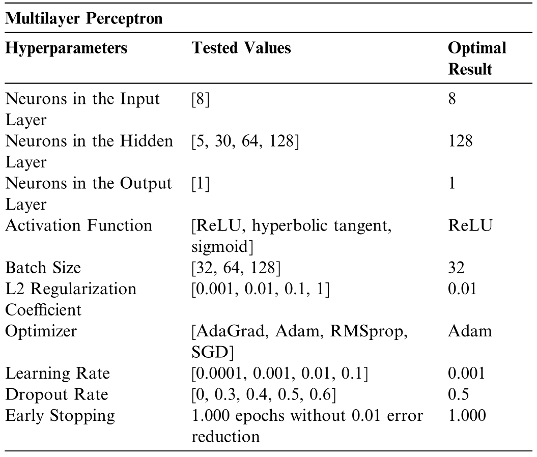
The input layer is defined by the dimension of the input data,which in this case consists of eight feat ures:historical generation,2-meter temperature,2-meter relative humidity,precipita tion,surface pressure,10-meter wind speed,100-meter wind speed,and 10-meter wind gust.The model has one hidden layer with 128 neurons,using the Rectified Linear Unit activation function.After the hidden layer,a dropout layer with a rate of 0.5 is added.The output layer of the mo del has a single neuron,as the goal is to predict a continuous value (regression),using the linear activation function,which is suitable for regression tasks.

The model is compiled using the Adaptive Moment Estimation (Adam) optimizer with a learning rateof 0.001.The loss function used is the mean squared error.During training,the batch size is set to 32,determining the number of samples propagated through the network before updating the parameters.The early stopping parameter is implemented to stop training if performance on the validation set does not improve after 1000 consecutive epochs,monitoring the validation loss.

The core of the XGBoost forecasting model is based on the ForecasterAutoreg class from the Skforecast library[27],for performing autoregressive forecasts.Additionally,the model uses XGBRegressor from Scikit-Learn [28].Cross-validation using the grid_search_forecaster function from skforecast.model_selection tested 451,584 different hyperparameter combinations (for each wind farm),with the configurations mentioned above identified as yielding the best results for the XGBoost model,minimizing overfitting and maximizing accuracy,according to the data in Table 5.The best choice for each hyperparameter is discussed as follows.

Table 5 Cross-validation tested for different hyperparameter combinations–eXtreme Gradient Boosting.

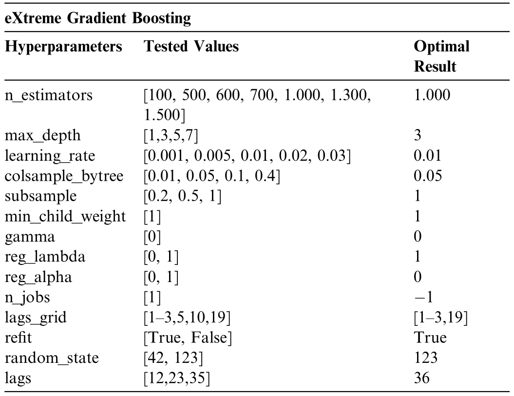
This model initialized with random_state set to 123 to ensure reproducibility of results and configured with 36lag s,indicating the consideration of 36 past values in the time series to fore cast future wind generation.Model optimization is perform ed through grid search,withthe hyperparameter n_estimators set to 1000,implying an ensemble of 1000 trees to mitigate overfitting while increasing model precision.The ma x_depth parameter is set to 3to prevent exc essive model complexity.The learning_rateis set to 0.0 1,balancing co nvergence speed and the risk of overshooting optimal solutions.

The colsample_bytree and subsample parameters are set to 0.05 and 1,respectively,controlling the fraction of features and samples used,affecting both model bias and variance.The min_child_w eight is set to 1,establishing the minimum sum of inst ance weights required for a split,and gamma is set to 0,specifying the minimum loss reduction needed to make a split,adjustable depending on the loss function.To reduce overfitting,the L2 regularization term (lambda) is set to 1,while the L1 regularization term(alpha)is set to 0,suitab le for high-dimensionalscenarios.The model also uses all available CPU cores for parallel computation,through the n_jobs parameter set to -1,increasing efficiency given the extensive data and complex calculations involved.The scale_pos_weight parameter is set to 1,useful in cases of high-class imbalance for faster convergence.

The exploration of lags is conducted using the lags_grid parameter,testing combinations of[1–3,19]to identify the temporal structure that best captures wind generation dynamics at the Pindaí complex.This is crucial for understanding how past values influence future predictions and for capturing seasonal patterns or other temporal dependencies.Finally,bootstrapping with 500 iterations helps estimate confidence intervals around predicted values,providing a measure of the model’s predictive uncertainty.

2.3 Predictive performance evaluation metrics

The evaluation of model performance corresponds to the accuracy and applicability of the predictive models.Inthis context,four metrics were used to assess the quality ofthe regression mod els: Kling-Gupta Efficiency (KGE),Mean Absolute Scaled Error (MASE),the Root Mean Squared Error (RMSE),and the Mean Absolute Error(MAE) [12,29].

KGE offers a comprehensive alternative that simultaneously assesses correl ation,mean bias,and relative variabilitybetween simulated and observed series.The motivation behind KGE is the explicit decomposition of error into three fundamental statistical components: correlational,representing the model’s ability to capture the temporal variability (synchrony) of the observed series;additive(mean bias),reflecting the systematic deviation between the means of the simulated and observed series;and multiplicative(relative variability),assessing the ratio between the dispersions (coefficients of variation) of the two series.It is calculated as shown in expression (6):

where r is the Pea rson correlation coefficient between the observed and sim ulated values,α is the ratio between the coefficients of variation of the simulated and observed series:  and β is the ratio betweenthe series averages:  A reduced KGE value can be decomposed to indicate whether the problem is related to low correlation (synchrony),mean under/overestimation(bias),or distortion in variability (amplitude of the modeled response) [12].

Mean Absolute Scaled Error (MASE) is a normalized error metric designed to evaluate the accuracy of a predictive model by comparing it to a simple naïve forecast.Unlike traditional error metrics such as MAE or RMSE,MASE provides a standardized way to compare forecasting performance across different datasets and time series with varying scales.It is particularly useful when working with time-series data,as it accounts for inherent seasonality and trends [12],using expression (7):

where the denominator represents the mean absolute error of a reference model,usually a persistence forecast.The key advantage of MASE is that it enables direct comparison across different datasets and time series models.

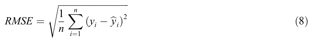
The Root Mean Squared Error (RMSE) measures the magnitude of a model’s predictions relative to the observed values,providing an intuitive understanding of model accuracy.The metric is calculated in three steps:first,the error differences are calculated by finding the difference between the observed value yi and the predicted value  for each data point,called the residual error.Next,each residual error is squared to avoid cancellation of positive and negative errors and to penalize larger discrepancies more severely [12].The mean of these squared errors is then computed,and finally,the square root of this mean is taken,resulting in the RMSE,as shown in formula(8):

The Mean Absolute Error (MAE) is a widely used statistical metric in predictive mode ling for evaluating the accuracy of forecast models .This metric measures the a vera ge of the absolu teerrors between the predictions and the empirically observed values [12].The mathematical expression for MAE is given by (9):

where n represents the total number of observations,yi is the observed actual value,and  is the predicted value.The metric measures the average magnitude of errors with-out considering their direction,treating both positive and negative errors equally.

3 Experimental results

The presentation of the results will be converted to MWmed,allowing for a direct comparison of the average energy generation capacity throughout the year by dividing the monthly values in MWh by the number of hours in the respective month.The months of January,March,May,July,August,October,and December have 744h.The months of April,June,September,and November have 720 h.February has 672 h.The forecast results compared to the actual generation can be seen in Figs.13–16.

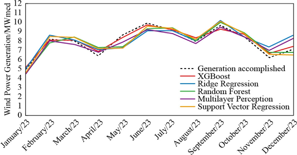
Fig.13.Wind Energy Forecast 2023 -Pindaí I.

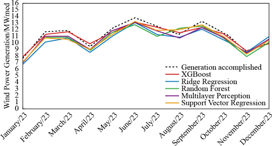
Fig.14.Wind Energy Forecast 2023 -Pindaí II.

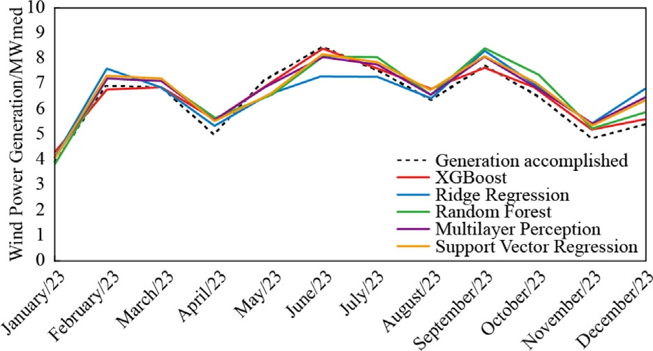
Fig.15.Wind Energy Forecast 2023 -Pindaí III.

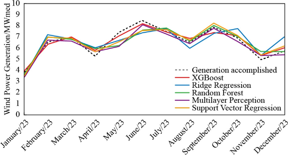
Fig.16.Wind Energy Forecast 2023 -PindaíIV.

Table 6 illustrates the average results of the evaluation metrics for all wind farms.The evaluation of machine learning models applied to wind power generation forecasting demonstrates a clear stratification in predictive performance across different methodologies.The Mean Absolute Scaled Error (MASE) values indicate that all models outperform a naïve benchmark,with XGBoost exhibiting the lowest error at 0.18,suggesting superior generalization and predictive capability.The Multilayer Perceptron (MLP) follows closely with a MASE of 0.29,reinforcing the ability of neural networks to capture non-linear dependencies in wind patterns.Conversely,Ridge Regression yields the highest MASE(0.41),suggesting that linear penalized regression struggles to accommodate the complexity of the dataset.

Table 6 Average results for all wind farms– evaluation metrics.

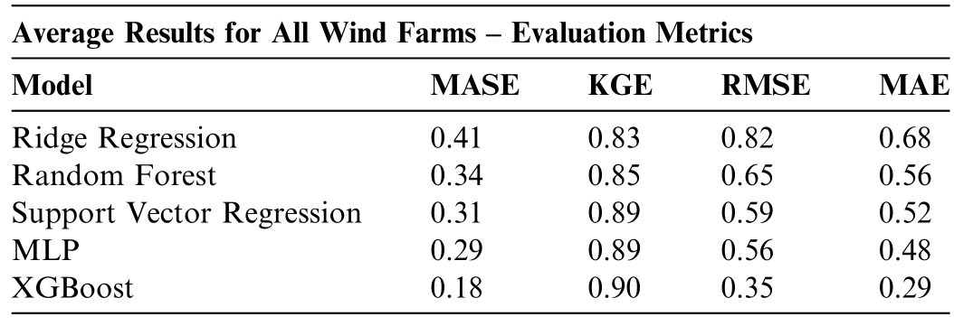
In terms of Kling-Gupta Efficiency (KGE),the results indicate that,particularly XGBoost,Support Vector Regression,and MLP Neural Network,achieved high KGE values (≈0.90),demonstrating strong predictive performance in capturing the statistical behavior of wind power generation across multiple wind farms.These models effectively reproduced the mean,variability,and temporal dynamics of the observed generation data,suggesting minimal bias and high reliability for operational forecasting.In contrast,simpler models such as linear regression showed comparatively lower KGE values,reflecting limitations in modeling the nonlinear and volatile natureof wind power.

Further supporting these observations,the Root Mean Square Error (RMSE) and Mean Absolute Error (MAE)reveal a consistent ranking across models,with XGBoost achieving the lowest RMSE (0.35) and MAE (0.29),reinforcing its efficiency in minimizing both variance and absolute deviations.The MLP model again emerges as a strong contender,with RMSE (0.56) and MAE (0.48),surpass ing Support Vector Regression,Random Forest,and significantly outperforming Ridge Regression (0.82 RMSE;0.68 MAE).The RMSE results highlight the abilityof XGBoost to minimize large errors,an essential attribute for energy forecasting applications where extreme deviations can lead to suboptimal operational decisions.

The application of the Giacomini–White test,grounded in the Mean Absolute Scaled Error (MASE) metric,represents a highly sophisticated methodological approach to comparing the predictive ability of models forecasting wind generation.MASE is calculated as the ratio between the mean absolute error of a model’s predictions and the mean absolute error of a naive forecast,typically constructed from the differences between consecutive observations.This scaling permits a standardized comparison across models even when the underlying time series exhibit different levels and variances.

In the study at hand,data from four wind parks were forecasted using various techniques,including linear regression,random forest,support vector machine,MLP neural network,and XGBoost.The results indicated that XGBoost achieved the lowest MASE values (0.200,0.175,0.174,and 0.185 for each park,respectively),serving asthe reference model for subsequent comparisons.

The Giacomini–White test was applied by constructing aseri es of loss differentials,given by (10):

where L(·) denotes the loss function based on MASE and yt represents the observed value.Under the null hypothesis,that there is no difference in predictive accuracy between the models,the mean of these differentials should bezero.However,the test statistics obtained (for instance,values of 4.20,3.75,3.90,and 4.10 for the models compared in Pindaí I,with similar resul ts observed in the other parks) accompanied by extremely low p-values (ranging between 0.0001 and 0.0003)demonstrate that the observed differences are statistically significant and cannot be attributed to chance.Moreover,the robustness of the test is reinforced by its consideration of temporal dependence and inherent heteroscedasticity in the residuals.

4 Discussion

The integration of Big Data approaches,data engineering and advanced predictive modeling techniques directly responds to the growing demand in the electricity sector for tools capable of increasing the predictability of intermittent generation,especially in medium and large-scale wind projects.In this sense,the use of supervised algorithms such as eXtreme Gradient Boosting,Multilayer Perceptron,Support Vector Regression,Ridge Regression and Random Forests has allowed the exploration of different mathematical paradigms,from penalized linear modeling to ensemble methods and deep neural networks,to represent the dynamics of wind energy production under variable meteorological conditions.

Taylor diagrams in Fig.17,provide a compact and informative visual synthesis of the statistical quality of wind power forecasts generated by five supervised machine learning algorithms.Each diagram encodes,in polar coordinates,three fundamental metrics for predictive evaluation: the standard deviation (σ),the Pearson correlation coefficient (ρ),and the centered root-mean-square error(CRMSE),the latter being implicitly represented by the Euclidean distance to the reference observation point.From a technical perspective,the angular correlation(θ=arccos(ρ)) offers a measure of linear alignment between predicted and observed time series,with angles approaching zero indicating a high degree of temporal pattern fidelity.Across all wind farms,XGBoost and SVR consistently achieved correlations exceeding 0.95,resulting in minimal angular deviation and,consequently,high precision in capturing monthly generation fluctuations.This high correlation suggests that both models are particularly well-suited to internalize the dominant temporal structures of the local wind regime,even in the presence of meteorological noise.

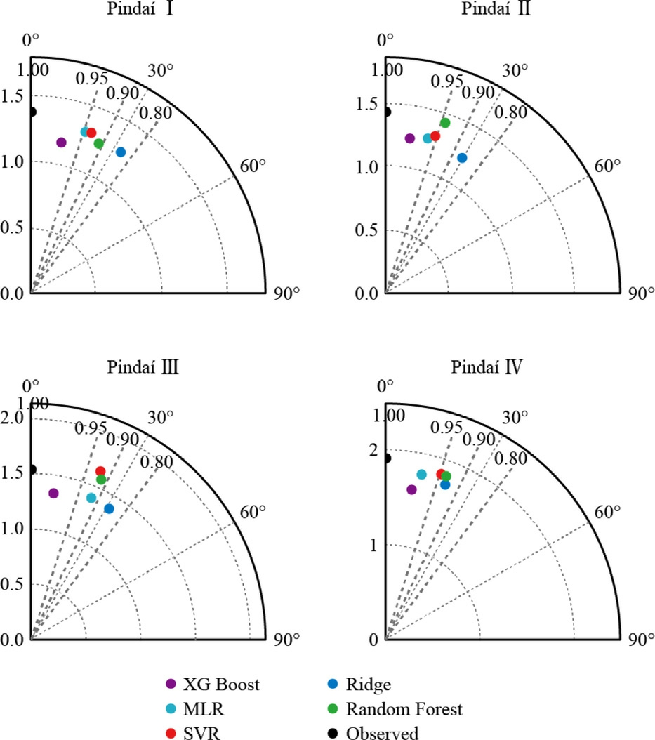
Fig.17.Taylor diagrams.

In terms of dispersion,the radial distances in the diagrams represent the standard deviation of the forecasts.Radial proximity to the observed series’ standard deviation—depicted by the central black dot—reflects the extent to which the model captures the empirical variability.Random Forest was observed to slightly overestimate the variance,placing its predictions marginally beyond the reference circle.This behavior may indicate heightened sensitivity to seasonal peaks or a tendency toward local amplitude overfitting.Conversely,Ridge Regression,despite achieving reasonably high correlation coefficients,exhibited a compressed variability —reflected in a smaller radial distance — indicating a structural bias inherentto its L2 penalization and linear assumption,which constrains the amplitude of predicted oscillations.

The CRMSE metric,implicitly represented by the Euclidean distance between the model points and the observed reference,reveals that XGBoost and SVR not only correlate well but also lie closest in magnitude and structure—particularly for Pindaí II and III.This demonstrates that,in addition to accurately mod eling the phase of the time series,these algorithms exhibit low unexplained residual dispersion,a hallmark of robust generalization.Furthermore,it is noteworthy that the diagrams for Pindaí III and IV present higher absolute amplitudes of standard deviation,reflecting intrinsically more volatile wind regimes.Nonetheless,the models maintain structural consistency,evidencing their multiscale adaptability.This predictive robustness can be attributed to the ensemble-based nature of XGBoost and Random Forest and the nonlinear mappings inherent in SVR and MLP,which are particularly adept at capturing complex effects such as atmospheric turbulence,pressure gradients,and topographic irregularities influencing wind power generation.

5 Conclusion

The findings of this research have significant relevance for the renewable energy sector,particularly in the field of wind power,where forecast accuracy directly impacts the operational efficiency and economic viability of projects.By increasing the accuracy of monthly wind power generation forecasts,the proposed methodology empowers engineers,operators,and investors to make more informed decisions,ultimately reducing operational costs and strengthening market competitiveness.

Building on the foundational work of Bouabdallaoui et al.[30]and Yin et al.[31],this study advances the accuracy and applicability of wind power forecasting techniques and integrates rigorous hyperparameter analysis through cross-validation and leverages high-resolution reanalysis meteorological models.In corporating meteorological variables as exogenous inputs further refines the machine learning models,ensuring that forecasts are robust and well-founded under realistic atmospheric conditions.

Beyond its predictive value for long-term energy planning,the modeling framework developed in this study presents substantial potential for real-time applications within the scope of smart grid infrastructures.The abilityof machine learning algorithms to capture complex,nonlinear relationships between high-resolution meteorological variables and actual wind power generation enables seamless integration into intelligent energy management platforms.In real-time environments,such predictive models can inform anticipatory control actions by forecasting short-term fluctuations in renewable energy output,thus enabling more effective demand response strategies,dynamic resource reallocation (e.g.,activating storage systems or dispatchable generation),and fine-tuned load balancing across the network.When coupled with supervisory control and data acquisition (SCADA) systems,these forecasts can support automated decision-making by providing predictive signals for grid operators,enabling the adjustment of setpoints,generation schedules,and reserve margins in advance of potential imbalances.Furthermore,integration into energy management systems (EMS) can optimize economic dispatch by minimizing the reliance oncostly spot market purchases or penalty charges due todeviations from contractual commitments.Ultimately,the operational deployment of these forecasting models can enhance grid reliability,improve supply–demand equilibrium,and foster the scalability of renewable energy within intelligent, style="font-size: 1em; text-align: justify; text-indent: 2em; line-height: 1.8em; margin: 0.5em 0em;">CRediT authorship contribution statement

Marcos V.M. Siqueira: Visualization,Project administration,Formal analysis,Resources,Methodology,Conceptualization,Investigation,Writing– original draft,Validation.Vitor H. Ferreira: Conceptualization,Writing–review &editing,Supervision. Angelo C.Colombini: Writing– review &editing,Supervision.

Declaration of competing interest

The authors declare the following financial interests/personal relationships which may be considered as potential competing inter ests: Marcos V.M.Siqueira is currently employed by Energy and Natural Gas Trading Company Tradener.

References

[1]ONS,Installed Generation Capacity -Dataset (2023) Availabel Online: https://dados.ons.org.br/dataset/capacidade-geracao.[accessed: Oct.2023].

[2]M.M.W.Lewis,M.Leithead,S.Galloway,Optimal maintenance scheduling for offshore wind farms,Renew.Energy (2018).

[3]E.Hossain,I.Khan,F.Un-Noor,et al.,Application of big data and machine learning in smart grid,and associated security concerns: a review,IEEE Access 7 (2019) 13960–13988.

[4]N.Cristianini,J.Shawe-Taylor,An Introduction to Support Vector Machines and Other Kernel-based Learning Methods,Cambridge University Press,Cambridge,UK,2000.

[5]A.J.Smola,B.Schölkopf,A tutorial on support vector regression,Stat.Comput.14 (3) (2004) 199–222.

[6]S.Haykin,Neural networks and learning machines,3rd ed.,Prentice Hall,2009.

[7]T.Q.Chen,C.Guestrin,XGBoost: a scalable tree boosting system,in: Proceedings of the 22nd ACM SIGKDD International Conference on Knowledge Discovery and Data Mining,ACM,San Francisco California USA,2016,pp.785–794.

[8]Open-Meteo.com (2024) Available Online: https://open-meteo.com/en/docs.[accessed: May 2024].

[9]A.E.Hoerl,R.W.Kennard,Ridge regression: biased estimation for nonorthogonal problems,Technometrics 12 (1) (1970) 55–67.

[10]R.Penrose,A generalized inverse for matrices,Math.Proc.Camb.Philos.Soc.51 (3) (1955) 406–413.

[11]L.Breiman,Random forests,Mach.Learn.45 (1) (2001) 5–32.

[12]T.Hastie,R.Tibshirani,J.Friedman,The Elements of Statistical Learning: Data Mining,Inference,and Prediction,Springer,2009.

[13]V.Vapnik,A.Y.Chervonenkis,A note on one class of perceptrons,Autom.Remote Control (1964).

[14]V.Vapnik,The nature of statistical learning theory,second edition,Priceedings of Statistics for Engineering and Information Science,2021.

[15]C.Cortes,V.Vapnik,Support-vector networks,Mach.Learn.20(3) (1995) 273–297.

[16]J.Platt,Fast training of support vector machines using sequential minimal optimization,in: Advances in Kernel Methods -Support Vector Learning,1998.

[17]H.Drucker,C.Burges,L.Kaufman,et al.,support vector regression machines,Advances in Neural Information Processing Systems,1 997.

[18]W.S.McCulloch,W.Pitts,A logical calculus of the ideas immanent innervous activity,Bull.Math.Biophys.(1943).

[19]P.J.Werbos,RegressionB,tNew Tools for prediction and analysis in the behavioral sciences,Harvard University,Cambridge,1974,Ph.D.dissertation.

[20]I.Goodfellow,Y.Bengio,A.Courville,Deep learning,MIT Press,Cambridge,2016.

[21]D.E.Rumelhart,G.E.Hinton,R.J.Williams,Learning representations by back-propagating errors ［ J］,Nature 323(6088) (1986) 533–536.

[22]A.Y.Ng,Feature selection,L1 vs.L2 regularization,and rotational invariance,in: Proceedings of Twenty-First International Conference on Machine Learning -ICML ’04,ACM,Banff,Alberta,Canada,2004,p.78.

[23]J.H.Friedman,Greedy function approximation: a gradient boosting machine.2001.

[24]L.Breiman,Bagging predictors,Mach.Learn.(1996).

[25]Scikit-learn (2023) Machine learning in Python.Availabel Online:https://scikit-learn.org/.[accessed: Oct.2023].

[26]Keras T (2023) Machine learning library.Availabel Online:https://www.tensorflow.org/guide/keras.[accessed: Oct.2023].

[27]XG Boost Documentation (2023) Availabel Online: https://xgboost.read thedocs.io/en/stable/.[accessed: Oct.2023].

[28]Skforecast Docs (2023) Availabel Online: https://skforecast.org/0.4.3/notebooks/forecasting-xgboost.html.[accessed: Oct.2023].

[29]T.Hong,P.Pinson,Y.Wang el al,Energy forecasting: a review and outlook,,Open Access J.Power Energy.(2020).

[30]D.Bouabdallaoui,T.Haidi,F.Elmariami,et al.,Application of four machine-learning methods to predict short-horizon wind energy,Global Energ.Interconnect.6 (6) (2023) 726–737.

[31]R.Yin,D.X.Li,Y.F.Wang,et al.,Forecasting method of monthly wind power generation based on climate model and long shortterm memory neural network,Global Energ.Interconnect.3 (6)(2020) 571–576.

Received 18 December 2024;revised 8 April 2025;accepted 26 May 2025

Abbreviations: Adam, Adaptive Moment Estimation; CERRA, Copernicus Regional Reanalysis for Europe; DWD, Deutscher Wetterdienst; ECMWF,European Centre for Medium-Range Weather Forecasts; FFNN, Feedforward Neural Networks; GBM, Gradient Boosting Machines; ITCZ, Intertropical Convergence Zone; MAE, Mean Absolute Errors; MASE, Mean Absolute Scaled Error; MBE, Mean Bias Error; MCAR, Missing Completely at Random;MLP,Multilayer Perceptron;MSE,Mean Squared Error;NOAA,National Oceanic and Atmospheric Administration;ONS,National System Operator;RMSE,Root Mean Square Errors;SMO,Sequential Minimal Optimization;SSTs,Sea Surface Temperatures;SVM,Support Vector Machines;SVR,Support Vector Regression;XGBoost,eXtreme Gradient Boosting

Peer review under the responsibility of Global Energy InterconnectionGroup Co.Ltd.

* Corresponding author.

E-mail address: marcos.siqueira@tradener.com.br (M.V.M.Siqueira).

https://doi.org/10.1016/j.gloei.2025.05.013

2096-5117/© 2025 Global Energy Interconnection Group Co.Ltd.Publishing services by Elsevier B.V.on behalf of KeAi Communications Co.Ltd.This is an open access article under the CC BY-NC-ND license(http://creativecommons.org/licenses/by-nc-nd/4.0/).

Marcos Siqueira holds a Bachelor’s degreein Electrical Engineering with an emphasis on Energy Systems from Universidade Positivo(2018),a Postgraduate degree in Financial Management,Costs,and Pricing from Universidade Positivo (2019),a Postgraduate degreein Power System Operation Coordination from Universidade Estadual de Campinas(Unicamp)(2021),and a Master’s degree from the Graduate Program in Electrical and Telecommunications Engineering at Universidade Federal Fluminense (UFF) (2024).Currently worksas an electrical engineer in the field of market intelligence and risk management at Energy and Natural Gas Trading Company Tradener.