0 Introduction

Energy demand forecasting is a critical aspect of modern power systems management,influencing decisionmaking processes in energy generation,distribution,and consumption [1].Accurate predictions are essential for ensuring energy reliability,optimizing resource allocation,and reducing operational costs.With the increasing complexity of energy systems and the growing reliance on renewable energy sources,demand forecasting has become more challenging due to the highly variable nature of patterns of energy consumption as well as environmental factors [2–6].Traditionally,a wide range of deep learning(DL) and machine learning(ML) models,such as Neural Networks (NN),Convolutional Neural Networks(CNN),and Long Short-Term Memory (LSTM) networks,have been applied to energy demand forecasting[7–9].Though these models have demonstrated promise,several problems still limit the advan cement of accurate and broadly applicable models [10–12].These challenges include small or insufficient datasets,repeated investigations with little novelty,and the inappropriate selection ofbaselines for comparison.Spe cifically,despite the demonstrated potential of CNN models in image recognition tasks [13,14],their application to tabular datasets,especially in energy demand forecasting,has not been sufficiently investigated or optimized.

This paper presents an innovative approach to overcome these limitations using a lightweight convolutional neural network (CNN),termed Tabular Lightweight CNN (TLCNN),specifically designed for tabular data.Unlike traditional CNN architectures,which are optimized for image processing [15,16],TLCNN adapts convolutional layers for structured data,making it wellsuited to handle the dynamic nature of energy demand forecasting.This model is competent to perform robust feature selection and is particularly effective in timeseries data pattern scenarios.TLCNN is designed to identify and prioritize relevant features from complex datasets automatically.The model is capable of evolving with changing data patterns,making it robust for timevarying energy demand predictions.The TLCNN structure ensures that the model remains computationally effi-cient even with large tabular datasets.In this study,we utilize the “BanE-16” dataset [17],which contains energy demand data influenced by meteorological factors such astemperature,wind speed,humidity,and precipitation.This dataset provides a comprehensive representation of the variables that impact energy demand,making it ideal toevaluate the performance of our proposed TLCNN model.We also compare the results of our TLCNN approach against various traditional machine learning algorithms,including Linear Regression[18,19],XGBoo st[20,21,22],and Random Forest[22–24]to demonstrate the efficacy of our model.

Several approaches have been explored to adapt deep learning models for tabular data.One study proposed an Image Generator for Tabular Data (IGTD),which transforms tabular data into images by mapping similar features close to each other in an image format,allowing CNNs to process them effectively [25].Another research effort analyzed neural network models like CharCNN,Bi-LSTM,and CNN+Bi-LSTM for semantic classification of tabular datasets,finding that Bi-LSTM performed best in terms of accuracy and confidence scores[26].A different study examined the effectiveness of the TabTransformer,a Transformer-based model designed for tabular data that leverages self-supervised learning to eliminate the need for labeled data and capturing intricate feature dependencies [27].While deep learning methods,particularly CNNs,struggle with small tabular datasets,some studies explored converting tabular data into images to apply transfer learning techniques,using methods such asSuperTML,IGTD,and REFINED approaches [28].Another study introduced the Dynamic Weighted Tabular Method (DWTM),which converts tabular data into images by dynamically embedding features based on their correlation with class labels.This allows CNN architectures like ResNet-18,DenseNet,and InceptionV1 to achieve high classification accuracy [29].However,these methods primarily focus on transforming tabular data into images rather than directly optimizing CNN architectures for tabular data.

While prior studies have demonstrated the effectiveness ofCNN-based methods for tabular data by transforming them into images,this introduces unnecessary complexity indata preprocessing and structure.These methods primarily generate visual representations of tabular data before applying deep learning models,which may not always be optimal.In contrast,our approach proposes a Tabular style="font-size: 1em; text-align: justify; text-indent: 2em; line-height: 1.8em; margin: 0.5em 0em;">Our research focuses on addressing the challenge of applying convolutional neural networks (CNNs) to tabular data for energy demand forecasting,a domain where traditional machine learning models have been predominantly used.The core research question driving this study is:Can CNNs effectively process tabular data directly and outperform traditional machine learning and deep learning models in energy demand prediction without the need for image transformation?

To investigate this,the study is guided by the following objectives:

1)To develop TLCNN,a lightweight CNN model tailored for tabular data processing.

2)Tocompare the predictive performance of TLCNN against wid ely used machine learning and deep learning algorithms,and

3)Toevaluatetheefficiency,accuracy,andgeneralization capability of TLCNN in energy demand forecasti ng.

The study is conducted in the context of energy demand forecasting,where accurate predictions play a crucial role in optimizing resource allocation and energy management.The methodology consists of two phases: in Phase 1,we design TLCNN to process tabular data directly by eliminating the need for image transformation that reduces computational complexity.In Phase 2,we compare TLCNN’s performance against three different machine learning algorithms to ensure a rigorous evaluation.The unit of analysis in this study consists of structured energy consumption records obtained from the uploaded dataset,which includes key attributes such as time-based energy usage,peak demand values,environmental conditions,and system load variations.By utilizing CNNs for tabular data without the need for transformation,this research aims to introduce a novel,more efficient approach to energy demand forecasting,demonstrating improved interpretability and predictive performance.

The rest of the study is structured as Section 2 reviews relevant studies in the area.Section 3 focuses on data processing,covering data acquisition,data prepossessing,and data augmentation techniques.Section 4 outlines the methods,providing an overview of the TLCNN model,the TLCNN algorithm,and CN N architecture,as wellas the ML algorithms used for comparison.Section 5 presents the results,including a discussion on model accuracy and efficiency,and a performance comparison between TLCNN and other ML algorithms.Section 6 covers the discussion.Finally,Section 7 concludes the study,summarizing key findings and potential future research directions.

1 Related work

The energy crisis is a major threat to national economies,inflicting extensive economic damage that stifles growth [30].A critical challenge is the negative impact on industrial development and output due to insufficient and unstable electricity supply[31].It is important to forecast the future need for energy to plan and manage production and distribution so that it doesn’t affect human life or the economy [32].It is also important to make sure the technique of foreca sting is efficient and more accurate[33].

To increase forecasting accuracy,numerous resear chers have developed a variety of load forecasting techniques[34].A study [35]investigates the possibilities of building energy management systems (BEMS) to optimize energy consumption while ensuring occupant comfort in contemporary buildings.The study employs a time series strategy employing long short-term memory (LSTM) networks for forecasting electricity consumption and refining model optimization.The results highlight the importance of optimization in enhancing prediction accuracy and suggest that future research with larger datasets could further refine these models.Another study [36]proposed a hybrid forecasting system to improve the precision and resilience of building energy consumption projections by fusing Long Short-Term Memory (LSTM) neural networks with Genetic Algorithms (GA).By employing GA,the model chooses LSTM hyperparameters such as the numberof layers,dropout rate,neurons,and learning rate in the best possible way.When the suggested approach was tested on actual educational buildings,it performed better than traditional LSTM models and other optimization methods including Bayesian optimization,grid search,and PSO.Its potential to enhance net-zero energy operations,facility decision-making,and building energy management is highlighted by the findings.However,both studies focus on deep learning models that require extensive optimization or hybridization.They do not explore lightweight CNNbased approaches that can directly process tabular data without transformation.This leaves a gap for efficient models suitable for real-time applications with limited computational resources.

For the purpose of forecasting electricity demand,another study [37]presents the Modified War Strategy Optimization-Based Convolutional Neural Network(MWSO-CNN),combining optimization techniques with CNNs to improve accuracy.MWSO-CNN performed better than techniques like GA/CNN,hLSTM,and CNN-LSTM when tested on a real-world dataset in cost value and mean squared error.Another study [38]proposes the EECP-CBL model,integrating Convolutional Neural Networks (CNN) and Bi-directional Long Short-Term Memory (Bi-LSTM) for electric energy consumption prediction using the IHEPC dataset.The model extracts spatial and temporal features through CNN and Bi-LSTM layers,enhancing predictive accuracy across different timeframes.Experimental results demonstrate that EECP-CBL outperforms state-of-the-art models suchas CNN-LSTM and LSTM in terms of MSE,RMSE,MAE,and MAPE.In addition,Fotis et al.[39]used artificial neural networks (ANNs) for foreca sting wind and solar energy production

in the Greek power system.While effective,their approach is limited to renewable-specific energy types and lacks a lightweight design for processing large-scale tabular datasets in general energy forecasting tasks.While most of these studies target energy consumption in buildings or renewable generation,our study distinctly focuses on structured electricity demand data collected from national power systems.

In Saudi Arabia,advanced statistical and machinelearning techniques are being developed to forecast the country’s annual electricity usage [40].Key factors like imports,GDP,population and refined oil products were identified.In this research optimized machine learning models (BOA-SVR,BOA-NARX) using Bayesian optimization and compared them with ARIMAX.In terms of forecasting accuracy (RMSE),BOA-NARX outperformed the other two models by 71% and 80%,respectively,compared to ARIMAX and BOA-SVR.This research[41]presents a study on forecasting peak electrical energy consumption in Togo combining ARIMA with LSTM and GRU.The ARIMA-LSTM hybrid model performed the best,achieving a root mean square error(RMSE) of 7.35,outperforming both the ARIMA-GRU hybrid (RMSE 9.60) and individual models (ARIMA,LSTM,GRU).The study highlights the effectiveness of hybrid approaches for more accurate peak consumption predictions,which can help utilities reduce costs and integrate renewable energy sources.

Recently,Alenizy and Berri [42]introduced the Novel Algorithm for Convolving Tabular Data (NCTD),which mathematically transforms tabular features into pseudoimage formats through enhanced spatial relationships such asrotation and reflection.This method enables CNNs to operate on transformed tabular data,demonstrating improved accuracy on several benchmark datasets.However,such transformations increase computational overhead and add complexity to data preprocessing.In contrast,the proposed TLCNN avoids artificial image generation entirely and directly structures tabular input for convolutional processing,reducing complexity while improving performance in energy demand forecasting tasks.

Future research should focus on expanding datasets to enhance model generalization and robustness,as larger datasets can help improve prediction accuracy and adaptability across diverse scenarios.Additionally,exploring advanced deep learning architectures such as Convolutional Neural Networks (CNN) and hybrid models can further refine forecasting performance.These advancements can be crucial for optimizing energy management systems,ensuring reliable infrastructure planning and supporting sustainable economic growth through precise demand forecasting.

2 Data processing

For this energy demand prediction using our proposed TLCNN model,we use the “BanE-16” [17]dataset which emphasizes the highest energy demand per day and peak consumption of energy.It considers factors like temperature range,wind,humidity,cloud cover,and precipitation.Our processing approach is focused on handling missing values,addressing outliers,augmenting data,and splitting the dataset for training and evaluation.We maintain dataset integrity by imputing missing values using the mode.Outliers are carefully examined and treated,particularly infeatures such as wind speed and temperature,to ensure that extreme values do not adversely affect model training.We employ data augmentation techniques to introduce variability in the weather-related data,simulating realworld fluctuations.To enhance the efficiency of training onkey features,we apply standardization to ensure consistent feature scales.Finally,the dataset is divided into training,validation and testing data,as shown in Fig.1,ensuring that the model can general ize well to new data.

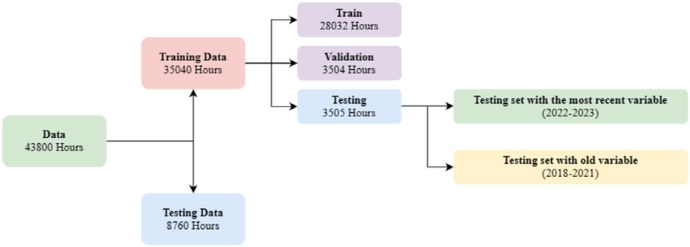
Fig.1.The dataset splitting into training and testing on different criteria.

2.1 Data acquisition

We collect daily peak energy consumption and demand data from the Bangladesh Power Development Board(BPDB),covering seven geographical zones from January 2018 to April 2023.These data are publicly available on the government’s official BPDB database,ensuring the authenticity and representativeness of actual national energy consumption.To complement this,we gather corresponding weather-related parameters from a meteorological station at Daffodil International University,which is equipped with calibrated sensors and specialized instruments.These include energy meters,smart meters,humidityhygrometers,thermocouples for temperature,anemometers for wind speed,ceilometers for cloud cover,and rain gauges for precipitation.This setup ensures that the data reflects real-world conditions and usage patterns.

The dataset offers a comprehensive view by combining environmental and energy consumption variables,making ithighly suitable for energy forecasting applications.Given the increasing pressure on national grids and the need for optimized resource allocation,our evaluation model addresses real-world challenges by improving demand prediction accuracy to reduce energy waste,enhance grid efficiency,and support sustainable energy planning.This makes the data and model highly relevant for practical implementation in smart grid systems and policy-level energy management.

2.2 Data preprocessing

In this research,we preprocess the dataset to ensure its integrity and appropriateness before training the model.The dataset comprises 1946 rows and 16 columns,containing features related to weather conditions and energy demand.Initially,redundant columns,such as ‘date_1’,‘date_2’,‘day’,‘month’,‘year’,‘temp2_ave(c)’,and‘wind_speed50_ave(m/s)’,are removed to reduce dimensionality and focus on relevant features.Missing values inkey columns,including total_demand(m/w) and max_generation(m/w),are imputed using the mode to preserve the integrity of the dataset while avoiding the influence of outliers on model performance.Additionally,data augmentation techniques are applied to introduce synthetic variations,which help enhance the model’s accuracy.Specifically,we use Gaussian noise [43]as the data augmentation technique to simulate real-world data variability and improve generalization.The total_demand(m/w)is chosen as the target variable for predicting electricity demand.We apply StandardScaler [44]to standardize the input features,ensuring the features have a standard deviation corresponding to one and a mean of zero.The standard variation is as follows in Eq.(1).

where μre presents the mean,and σdenotes the standard deviation of the feature values.After preprocessing,we normalize the target variable to diminish the riskof exploding gradients,which can adversely affect model stability.We’ve used min–max normalization here.The transformation is performed as follows in Eq.(2).

where is the normalized value,x is the original value,max is the maximum value and mi nis the minimum value in the dataset.The dataset is divided into training,validation,and testing sets.The dataset is split as follows:2490 instances were used for training,623 instances for validation,and 779 instances for testing.These splits were used consistently across model training,validation monitoring,and final evaluation.Finally,the data is reshaped to fit the input requirements of the TLCNN model,using the shape to align with the convolutional neural network’s architecture.

2.3 Data augmentation

Augmenting data [45]is a fundamental approach used to enhance model performance and generalization,particularly when working with limited or imbalanced datasets.Adding variability to the training data helps models become more adaptable and less prone to overfitting.In this study,we use a crucial technique called “Gaussian noise augmentation” [46,47]to increase the model’s resilience and enhance its capacity to generalize to new data.By adding controlled noise to the dataset,the modelis encouraged to learn more robust patterns,which lowers the chance of overfitting and increases stability all around.This section delves into the reasoning and methodology behind the implementation of data augmentation ina regression task.A tabular dataset [48]is fed intoa Convolutional Neural Network (CNN) and data augmentation techniques are combined to assist the model in better representing intricate relationships in the data.The rationale for using these techniques,particularly “Gaussian noise augmentation”,is further explored in the context of improving predictive accuracy and generalization.

Gaussian noise is characterized by its normal distribution around a mean of zero with a specified standard deviation.In this study,we have applied Gaussian noise witha standard deviation of 0.01 to each numerical feature in the dataset.The mathematical formulation for the noise addition process is given by Eq.(3).

In this Equation,is the augmented data point,x re presents the original data,is the Gaussian noise sampled from a normal distribution where σdenotes the standard deviation.This augmentation techniqueis applied to all numerical columns in the dataset,effectively creating additional training samples with slight deviations.By adding noise,the convolutional layers are encouraged to extract robust feature representations that are not overly sensitive to minor fluctuations in the input data.This is critical in a regression task where the objectiveis to predict continuous values.The ability to generalize well under slight variations is a valuable property that enhances the model’s predictive performance and reliability in practical implementations.

2.4 Reshaping and structuring data for CNN input

Convolutional Neural Networks are traditionally designed for image-based inputs.Since this study utilizes a tabular dataset,the data is reshaped into a threedimensional 32323format to make it compatible with CNN processing.After performing essential data preprocessing steps—including feature selection,dimensionality reduction,handling missing values,feature scaling,and data augmentation—the preprocessed data is restructured into a matrix format that preserves spatial relationships among energy-related attributes.To further enhance feature representation,numerical features are stacked across three channels,allowing CNN layers to capture multidimensional dependencies within the tabular dataset.This structured representation enables TLCNN to leverage convolutional layers for feature extraction,capturing hidden correlations between meteorological variables and energy demand patterns.This structured representation enables TLCNN to effectively extract complex feature interactions through convolutional layers,uncovering hidden correlations between meteorological variables and energy demand patterns,ultimately improving forecasting accuracy.

2.5 Optimal variables selection for experiments

The dataset comprises various columns representing features and attributes in Fig.2,with each row corresponding to a specific variable such as temperature,pressure,wind speed,precipitation,energy demand,and generation.Energy demand is closely influenced by temperature,as warmer conditions lead to increased use of air conditioning Energy demand is closely influenced by temperature,as warmer conditions lead to increased use ofair conditioning and subsequently increased energy consumption.Conversely,c older weather leads to higher demand for heating.Changes in temperature influence overall energy consumption patterns as well,with hotter orcolder weather typically corresponding to higher peak demand periods.Predicting pressure changes facilitates short-term weather forecasting,which directly influences energy consumption patterns.Precipitation,whether in the form of rainfall or snowfall,also affects energy demand.

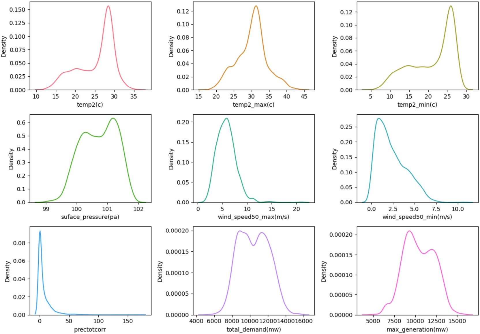
Fig.2.Environment-related variable visualization for energy demand.

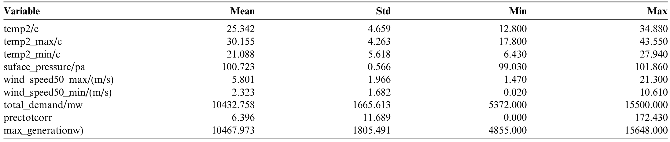
Heavy rainfall may reduce outdoor activities,decreasing the need for lighting,while snowfall can increase heating requirements.Accurate predictions of precipitation help adjust energy supply in response to changes in demand.Incorporating these weather-related factors into forecasting models enables more thorough predictions of electricity demand and supply trends.Such forecasts are essential for maint aining grid stability,optimizing energy production,and reducing costs.Efficient forecasts enable efficient energy resource allocation by considering the interactions between weather conditions,consumption behaviors,and generation capacities Upon considering all these criteria,we select optimal variables by measuring descriptive statistics as shown in Table 1.

Table 1 Environment-related variable selection for energy demand.

3 Methods

In this section,we detail the methodology employed to develop and evaluate our proposed Tabular Lightweight Convolutional Neural Network (TLCNN) for energy demand prediction using structured tabular data.We begin by outlining the TLCNN architecture,focusing on data preprocessing,model training,and performance evaluation.The TLCNN algorithm is then described,highlighting the adaptation of convolutional neural networks—traditionally used for image data—to effectively process tabular datasets.We further elaborate on the CNN architecture,including data reshaping,convolutional and pooling layers,and the use of dense layers for regression tasks.Finally,we compare the performance of TLCNN with traditional machine learning models to assess its effectiveness in forecasting energy demand.

3.1 Outlines of TLCNN

Fig.3 depicts our proposed TLCNN architecture,which is designed to handle tabular data effectively by transforming it into a format suitable for convolutional operations.In the first phase,we focus on preprocessing the tabular data,which involves two main steps: Data Cleaning and Data Labeling.During Data Cleaning,we structure the raw data by filtering out any inaccuracies,inconsistencies,or missing values to ensure that the dataset is reliable.Once the data is cleaned,we proceed to Data Labeling,where we categorize and assign labels to the data points,creating a labeled dataset.The training and testing subsets of this labeled dataset are then separated,which will be used for training the model and evaluating its performance.In the second phase,we experiment with various machine learning techniques to evaluate their effectiveness in predicting energy demand.We implement different models,analyzing their strengths and weaknesses based on performance metrics like accuracy and error rates.Next,we move to the third phase,where we experiment with the Tabular Lightweight CNN (TLCNN)model.This phase involves training the TLCNN on the same training dataset,allowing us to evaluate how well itcaptures complex data patterns.In the fourth phase,wecompare the TLCNN’s performance with that of the traditional machine learning models.This comparison helps us identify which approach yields better results in terms of accuracy,Mean Squared Error(MSE),and other relevant metrics.Finally,we analyze the results to determine which model performs best on structured tabular data.This comprehensive evaluation enables us to draw meaningful conclusions about the effectiveness of each model in the context of energy demand forecasting.

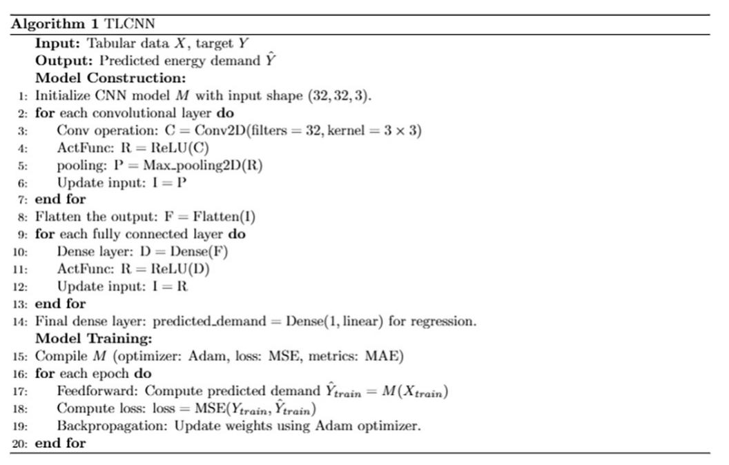
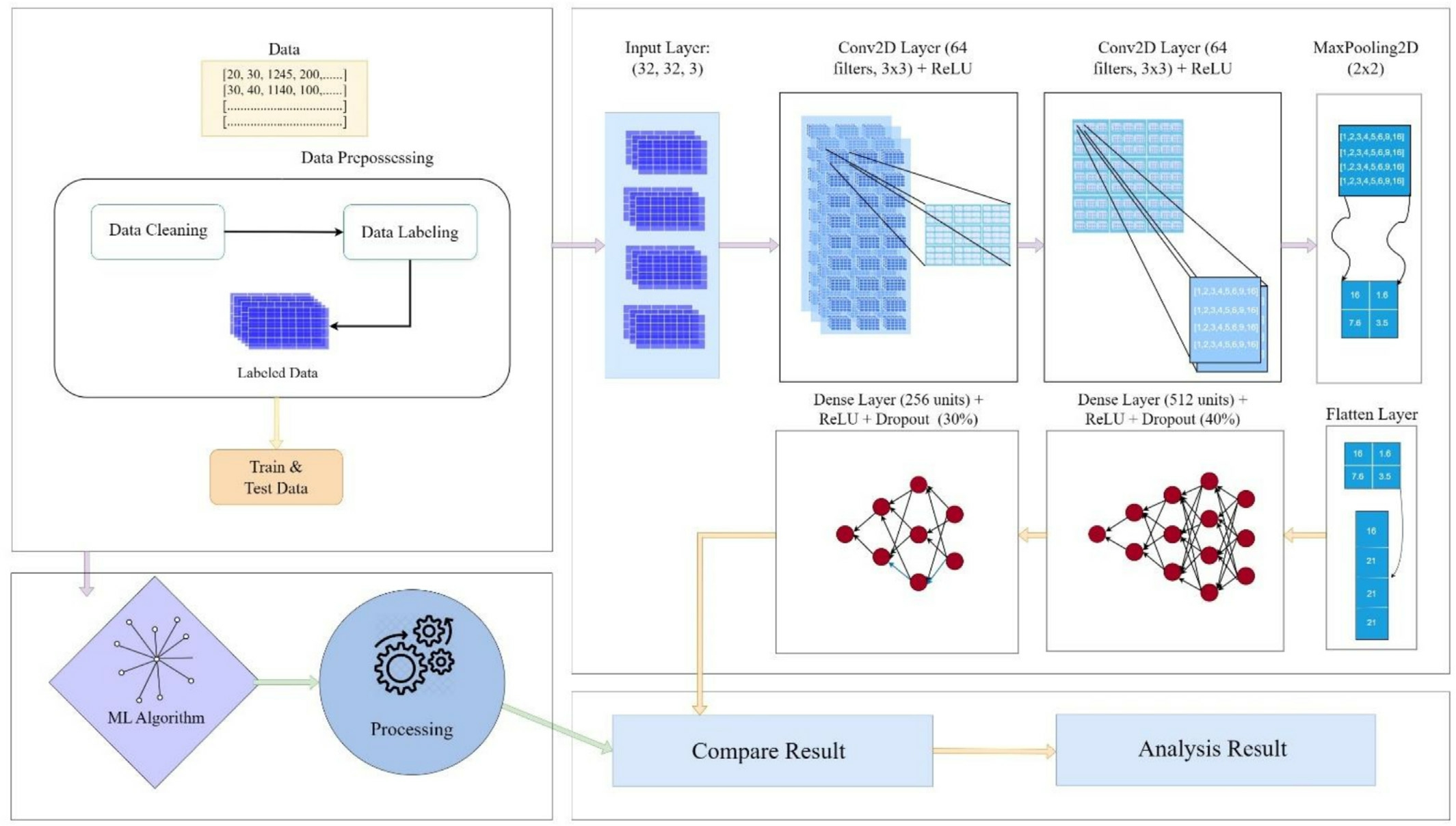
Fig.3.Overall visualization of the TLCNN model.

3.2 TLCNN algorithm

Convolutional Neural Networks are traditionally designed for image data but in our case,we apply CNN toa tabular dataset,which presents a unique challenge.Toaccomplish this,we present an entirely novel,modified CNN architecture called TLCNN that is designed specifically for tabular data in Algorithm 1.We take tabular data X and the target variable Y as inputs to the TLCNN model.Initially,we reshape the data into a 3D format32323to adapt it to the CNN architecture allowing for the prediction of energy demand .After initializing the model M,we perform multiple iterations of convolution operations using a 33 kernel size,applying multiple layers of convolution.To introduce non-linearity,the activation function named ReLU is applied after each convolutional layer,helping to solve issues like vanishing gradients.We deploy max-pooling layers after the convolution operations to reduce the dimensionality of the feature maps and emphasize important features.After that,weapply a flatten layer to the convolutional operation’s output,transforming the multi-dimensional feature maps into a vector in one dimension.This phase involves preprocessing the data to ensure it is properly formatted and optimized for input into the dense,fully connected layers.Each iteration involves adding a dense layer in the fully connected layers followed by the ReLU activation function.Finally,a Dense layer with a single output neuron is added for the regression task,using a linear activation function to predict the energy demand.The Adam optimizer is used to compile the model,and the evaluation metric is Mean Absolute Error,while the loss function is Mean Squared Error.During training,we perform feedforward passes to compute the predicted energy demand for the training data and calculate the training loss using Mean Squared Error.Backpropagation is employed to update the model weights iteratively in each epoch.

3.3 CNN architecture

A Convolutional Neural Network(CNN)[49]is a deep learning architecture primarily used for processing gridlike data such as images.It automatically learns to detect important features such as edges,textures,or objects through convolutional filters,reducing the need for manual feature extraction.Our proposed model,the Tabular Lightweight CNN (TLCNN),is a lightweight convolutional neural network architecture specifically designed tohandle structured tabular data.It adapts principles from traditional image-based CNNs for regression tasks.Following some preliminary fine-tuning,we configured this customized architecture for energy demand prediction using tabular data as illustrated in Fig.4.Table 2 provides acomprehensive summary of the model parameters and all relevant information.

Table 2 TLCNN parameter information.

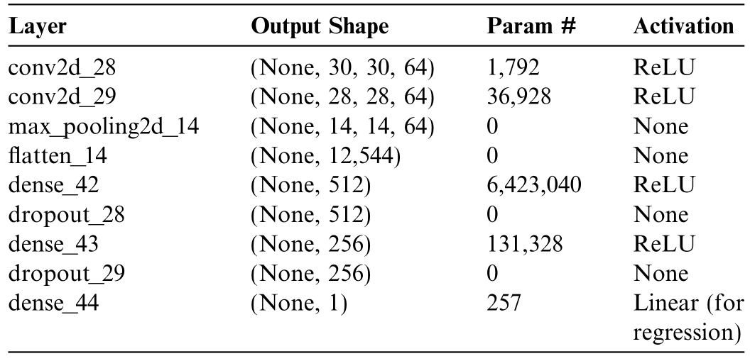
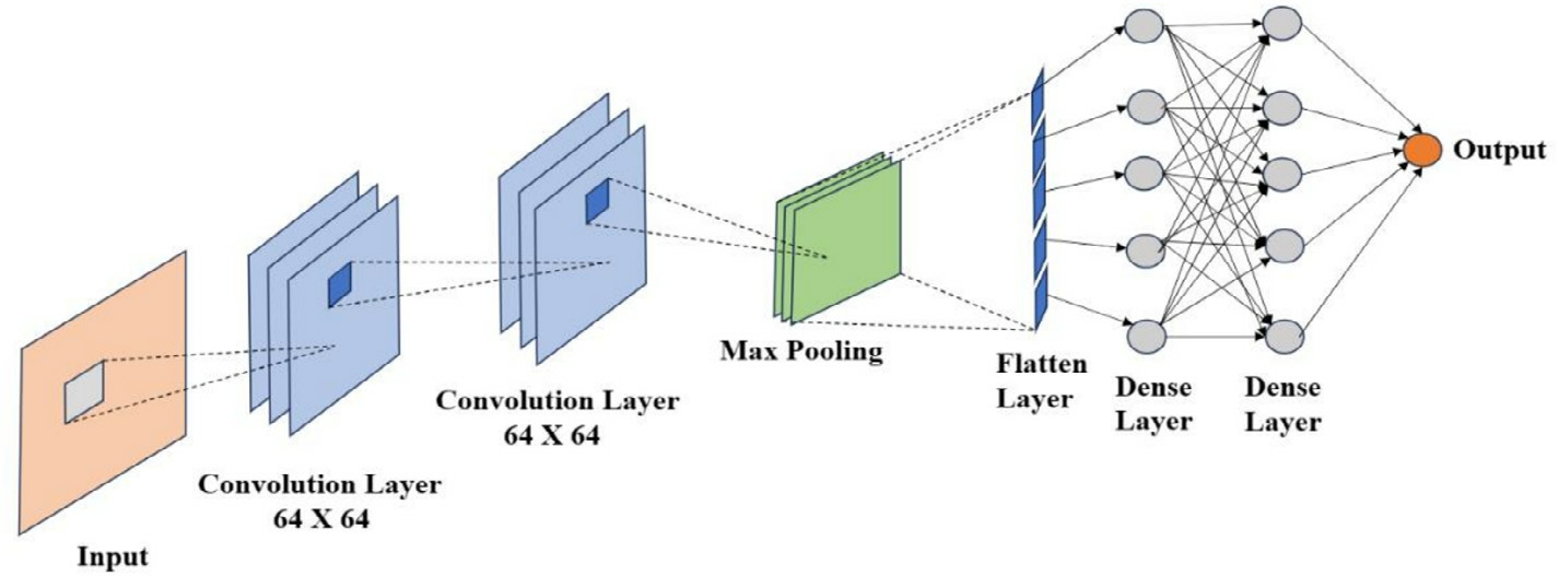
Fig.4.TLCNN model convolutional neural network architecture.

1) Input Lay er

The TLCNN expects input data in a reshaped form,typically of size 32323,mimicking the structure of image-like data.Tabular data is reshaped into this 3D format to allow convolutional layers to process it effectively.The reshaping begins with the origin al tabular data D,which has a shape (m,n),where m represents the number ofrows (samples) and n is the number of columns(features).General formula of reshaping is stated in Eq.(4).Tomatch the expected input shape of the CNN,the data needs to be transformed into a tensor with dimensions

The total number of elements in the original data matrix D must equal the total number of elements in the reshaped form.That is,the product of m and n must equal the product of the target dimensions hwc323233072.

That can be expressed as Eq.(5):

In cases where m n is less than 3072,paddingisrequired.This involves adding zeros to the data until the total number of elements matches 3072.The amountof padding needed,denoted by p,is given by Eq.(6) and the padded data is expressed in Eq.(7).

Conversely,if m n exceeds 3072,truncation is performed by removing excess eleme nts from the original data as expressed in Eq.(8).

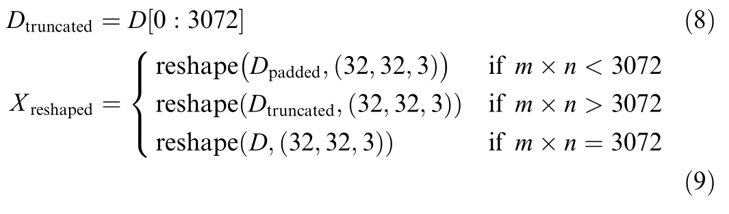
Equation (9) formalizes the process of transforming tabular data into a 3D tensor suitable for TLCNN.The padding ensures that smaller datasets are expanded to the required size,while truncation reduces larger datasets to fit the target shape.In both cases,the resulting tensor is shaped as 32323which allows the CNN to process the tabular data effectively.

2) Convolutional Layers

The architecture begins with two convolutional layers,each equipped with 64 filters and a 3 3kernel size.Every layer is followed by ReLU activations,which allow the network to detect complex patterns and introduce nonlinearity in the provided data.The input image is described by a tensor A of dimension h1 w1 c1,where h1 is the height of the image,w1 the width,and c1 represents the number of channels denoted in Eq.(10).Each filter B in the convolutional layer is a tensor of size p1 q1 c2,where p1 and q1 represent the filter dimensions,and c2=c1,the number of input channels denoted in Eq.(11).

When the convolution operation is performed between the input tensor A and filter tensor B,it yields a feature map D,the dimensions of which are reduced relative to the input due to the receptive field size of the filters.The dimensions of the following feature map are calculated using Eq.(12).di

This equation reflects the size of the output when a filter slides over the input without padding [50]and usinga stride of 1.Each subtraction accounts for the reduction in traversable positions due to the spatial size of the filter and the added 1 represents the initial alignment where the filter starts at the top-left corner.The reduced output size ensures that only positions where the filter fully overlaps the input are considered in the convolution.

The actual value of the feature map at a spatial locationijis computed by taking a localized patch of the input and performing an element-wise product followed bya summation over all dimensions.This operation canbe mathematically expressed through Eq.(13) which denotes the convolution at a specific spatial location ij.The detailed computation of this operation is expanded in Eq.(14),where the summation iterates over the spatial dimensions and depth of the filter to perform element-wise multiplication and aggregation across the receptive field.

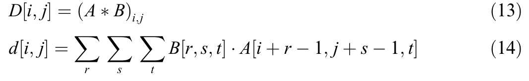
The triple summation iterates over the height r widths and depth tof the filter.For each position,the filter weights are multiplied by the corresponding values in the re ceptive field of the input tensor.The shifted indice salign the filter appropriately over the input patch.This operation extracts local features,such as edges or textures,depending on the learned weights of the filters.

Following the convolution,the outpu tFis passed through a max pooling layer [51]to downsample the feature maps.This step retains only the most prominent features in localized regions.It effectively reduces the spatial dimensions while preserving significant information.The output from the convolution is shown in Eq.(15) and the result after applying max pool ing is shown in Eq.(16).The convolution processes the input using a filter,while max pooling reduces the size of the feature map by keeping the most important values.

The function ψq denotes the max pooling operator appliedto the convolution output.Maxpoolingisawidely used down sampling technique that selects the maximum value within a defined pooling window,thereby retaining the strongest activation in each local region.This operation serves to reduce computational burden and control overfitting while maintaining robustness against small translations.

The spatial dimensions of the pooled outpu tGare determined by the size of the pooling kernel,the stride used for window movem ent and any padding applied to the input feature map.The output dimensions are computed in Eq.(17).

Here,a1a2,are the spatial dimensions (height and weight) of the input to the pooling layer,b1b2 are the height and width of the pooling kerne l,drepresents the amount of zero-padding applied around the borders of the input and tdenotes the stride length that determines how far the window moves during pooling.The parameter acrefers to the number of channels in the feature map and remains unchanged during the pooling operation.The formula ensures precise control over the size of the pooled output,particularly when the input dimensions are not evenly divisible by the pooling parameters.Padding d helps preserve the spatial structure while stride tgoverns the extent of spatial down sampling.Together,these operations—convolution followed by max pooling—allow the network to learn spatial hierarchies of features,reduce the volume of data for subsequent layers and improve the overall efficiency and effectiveness of the architecture.

3)Flattening Layers

After the feature extraction stage,the output is flattened into a 1D vector.This transformation prepares the data for full y-connected layers,which are more suitable for decision making and prediction tasks,as shown in Fig.5.

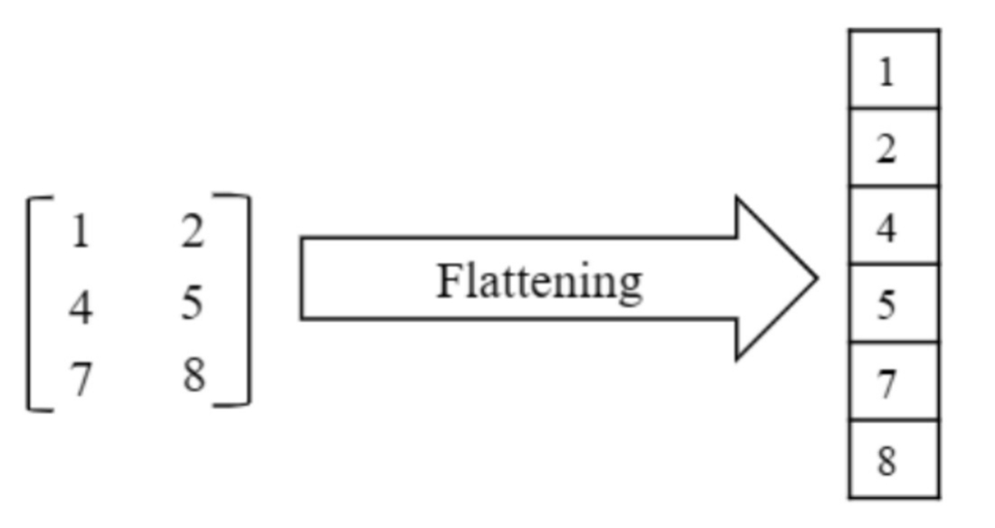
Fig.5.Flattening a 3 2 matrix into a 1D vector by rearranging elements row-wise.

4)Dense Lay ers

A fully connected layer,also referred to as a dense layer,is a critical element in artificial neural networks(ANNs).It performs a linear transformation followed by anactivation function,enabling the model to learn from the input data and make predictions.The layer operates bycomputing a weighted sum of the inputs,where each input is multiplied by a corresponding weight,and the result is summed with an additional bias term.This process allows the model to adjust the importance of each feature during training.The mathematical representation of the fully connected layer is expressed in Eq.(18).

In the equation,z rep resents the weighted sum,where wi are the weights assigned to each input xi,and b isthe bias term.The number of inputs is denoted by n,highlighting that each input is independently processed and has a corresponding weight,which determines its influence on the network’s decision-making process.Once the weighted sum is computed,an activation function is applied to introduce non-linearity.Without this non-linearity,the network would remain apurely linear model,unable to capture complex relationships in the data.The activationfunction transforms the output of the weighted sum,and this transformation is mathematically described in Eq.(19).

Here,a re fers to the activated output,and fis the activation function.One of the most commonly used activation functions in neural networks is the Rectified Linear Unit (ReLU),defined in Eq.(20).

ReLU effectively sets all negative values to zero while retaining positive values,thereby helping the model capture complex patterns in Fig.6.

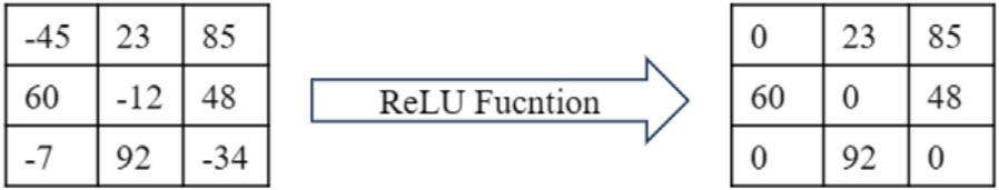
Fig.6.Applying the ReLU activation function to a matrix.Negative values are set to zero,while positive values remain unchanged.This operation introduces non-linearity and allows the model to better capture complex patterns in data.

To address the issue of overfitting in neural networks,Dropout is used as a regularization technique.Dropout layers randomly deactivate a certain pro portion of neurons during each forward pass of training.Mathematically,this can be represented like Eq.(21).

where r is the dropout rate and a is the activation output from the previous layer.The dropout rate r determines the fraction of neurons that will be dropped,typically chosen as values between 0 and 1.By preventing neurons from becoming overly specialized during training,dropout helps improve the model’s ability to generalize.

In our proposed model,two fully connected layers are incorporated to refine and aggregate the features extracted by earlier convolutional layers.The first fully connected layer consists of 512 neurons and applies ReLU as the activation function which ensures that the network learns nonlinear relationships in the data.This layer serves to combine and further abstract the features learned in the convolutional layers.To reduce the risk of overfitting,a Dropout layer with a rate of 0.3 is introduced,randomly deactivating 30% of the neurons during train ing.Dropout regularization is essential for preventing the model from becoming too reliant on any specific subset of neurons,enhancing its ability to generalize to unseen data.Following this,the second dense layer contains 256 neurons and also uses ReLU as its activation function.This additional layer further refines the feature representations and introduces another Dropout layer with a rate of 0.2,randomly deactivating 20% of the neurons during training.The inclusion of these Dropout layers ensures that the model remains robust and reduces the chance of overfittingas the network deepens.

5) Output Layer

In the final stage of the model,a single neuron is utilized in a dense configuration with a linear activation function,which is particularly well-suited for regression tasks requiring continuous,real-valued outputs.This function is based on the familiar equation of a straight line,

which can be generalized for multiple input features ina neural network context.The output of the final layeris formulated as Eq.(23).

where,y is the predicted output corresponding to the linear combination of inputs,wi represents the learned weights for each input feature xi (analogous to the slope in linear regression),bis the bias term,serving as the intercept,and αis a scaling factor or activation coefficient applied to the weighted sum of inputs.

This property is especially beneficial in regression tasks,as the predicted outputs remain continuous and unbounded making it suitable for applications suchas price predictions,temperature forecasting,and other scenarios requiring real-valued outputs.Consequently,the final linear layer facilitates continuous output by computing a weighted sum of features extracted from preceding layers without any non-linear transformation.The incorporation of this linear activation function is critical for regression problems,as it enables the model to generate predictions without constraints on the output range while benefiting from the complex feature representations learned by earlier layers through non-linear activations like ReLU.

3.4 Machine learning algorithm

Machine learning is a branch of AI (artificial intelligence) that emphasizes the growth of statistical models and algorithms that allow computers to gain knowledge from data and make intelligent decisions or predictions.In our work,we are testing our dataset using several machine learning algorithms,particularly from the supervised learning category,which relies on labeled data to train models.

1) XGBoost

XGBoost [52]is a highly efficient and scalable ensemble learning algorithm that employs a gradient-boosting framework.It sequentially constructs an ensemble of decision trees,with each new tree focusing on correcting the errors made by the previous ones as depicted in Fig.7.This iterative process,known as gradient boosting,allows XGBoost to build a strong predictive model by leveraging the collective wisdom of multiple weak learners XGBoost optimizes a loss function that calculates how much the actual values depart from the predicted values.In addition tothe loss fun ction,XGBoost incorporates regularization techniques to avoid overfitting and enhance generalization performance.This is achieved by penalizing complex modelsand encouraging the algorithm to find simpler,more interpretable solutions.The prediction of an XGBoost model is given by Eq.(24).

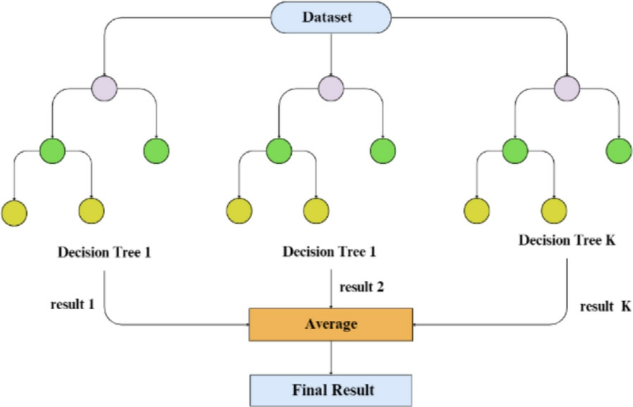
Fig.7.XGBoost model visualization.

where  the predicted value for the i-th data point,K is the number of trees,fk is the k-th tree,and F represents the space of regression trees.The final prediction of the XGBoost model is obtained by summing the contributions of all individual trees,adjusted by the learning rate.

2) Random Forest

The Random Forest (RF) [22]model is a technique of ensemble learning that constructs a large number of decision trees throughout the training stage.The original data is randomly selected for each decision tree’s training,using a subset of characteristics chosen at random for every node as illustated in Fig.8.Adding variety to the individual trees,it lowers the possibility of overfitting and enhances prediction accuracy overall.

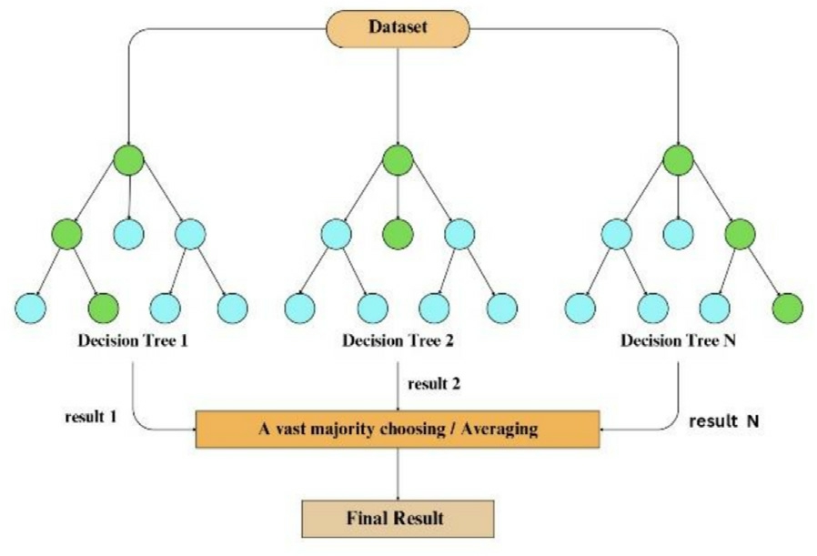
Fig.8.Random Forest model visualization.

The output of the RF model is obtained by aggregating the predictions of all individual trees.When it comes to classification problems,the final prediction is the class that most trees choose.For regression tasks,the median or average prediction of the individual trees is returned.We can denote the Random Forest (RF) model as Eq.(25),

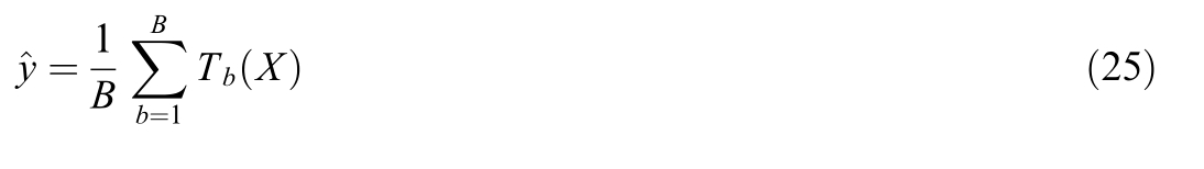
where Xis the input data,B is the number of decision trees in the ensemble,is the prediction of the bth decision tree.

3) Multiple Linear Regression

Multiple linear regression[18]is a statistical method for modeling and analyzing the connection between two or more independent variables and a dependent variable.This method extends the concept of simple linear regression,which involves only one predictor,to cases with multiple predictors.The primary objective of multiple linear regression is to identify the linear equation that best captures the way the independent factors interact to affect the dependent variable.This approach is extensively utilized to comprehend and forecast results in a variety of disciplines,such as social sciences and economics based on several influencing factors.The general Equation of multiple linear regression.

In this Eq.(26),y i is the dependent variable (the outcome being predicted) for the i-th observation,x1i,x2i,,x ni are the independent variables (predictors) for the ith observation,β0 is the intercept of the regression model,β1,β2,,βn are the regression coefficients,representing how each independent variable affects the dependent one,∊ iis the error term for the ith observation,accounting for the discrepancy between the observed and predicted values.Despite its effectiveness,multiple linear regression has boundaries.It presumes that there is a linear relationship between the dependent and independent variables,which may not always capture complex,non-linear relationships.This limitation can lead to suboptimal predictions if the true relationship is non-linear.The model’s performance is evaluated by minimizing the total sum of squares,which involves reducing the sum of the squared deviations of the values that were observed from the predicted values.This can be expressed mathematically(Eq.(27),

where y k is the actual value for observation k,y is the mean of all observed values,is the predicted value from the regression model for observation k.Multiple linear regression is an essential analytical tool for examining and forecasting outcomes by considering multiple predictors,offering critical insights into how different factors impact the dependent variable.

3.5 Experimental setup

This section details our TLCNN environment setup with Tensor Flow.The models are executed on a computer system that has an Intel(R) Core(TM) i5-1070 K CPU running at 3.70 GHz and 16 GB of RAM.With a batch size of 16 and a validation split of 0.2,we train the model across 200 epochs using the Adam optimizer.Throughout the training process,the learning rate is kept constant at 0.001.

4 Result analysis

This section presents the results of the TLCNN model and compares its performance with conventional machine learning and deep learning models.The evaluation is based on Mean Squared Error (MSE) and Mean Absolute Error(MAE). A comparative analysis highlights the strengths and weaknesses of TLCNN against traditional machine learning algorithms,including Linear Regression,XGBoost,and Random Forest and deep learning algorithms including LSTM and Bi-LSTM.Additionally,various visualizations offer insights into model efficiency,training dynamics,and prediction accuracy.

4.1 Model performance and generalization

The proposed TLCNN model’s performance is assessed in comparison to standard machine learning and deep learning (RNN) algorithms.Table 3 presents a detailed evaluation of training accuracy,test accuracy,and error metrics (MSE and MAE) for each model.

Table 3 Performance evaluation.

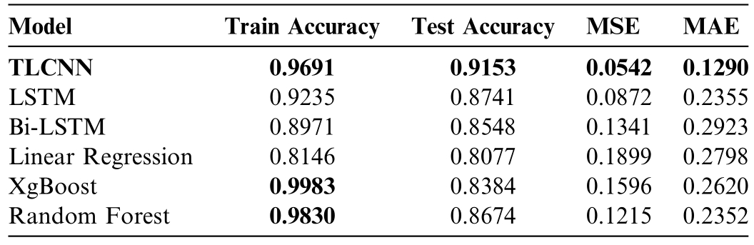
TLCNN achieves the highest test accuracy of 0.9153 while maintaining low error rates (MSE: 0.0542,MAE:0.1290).This suggests that the model effectively generalizesto unseen data while minimizing prediction errors.In contrast,Linear Regression demonstrates the weakest performance,with a test accuracy of 0.8077 and the highest error rates.XGBoost achieves a near-perfect training accuracy of 0.9983 but exhibits overfitting,as reflected in its significantly lower test accuracy of 0.8384.Random Forest performs moderately well,balancing accuracy and error minimization,though it does not surpass TLCNN in terms of generalization.The training times for the baseline models are as follows: Linear Regression required approximately 40 ms,XGBoost took around 194 ms,and Random Forest required approximately 1.07 s.LSTM and Bi-LSTM models show better test accuracy (0.8741 and 0.8548) and lower error rates compared to Linear Regression and XGBoost,indicating their strength in capturing temporal patterns;however,they still lag behind TLCNN in both accuracy and error minimization,especially in handling high-dimensional tabular features.

Fig.9 provides a comprehensive comparison of test accuracy across TLCNN,traditional machine learning models (Linear Regression,XGBoost,Random Forest),and deep learning-based recurrent models (LSTM and Bi-LSTM).TLCNN achieves the highest accuracyat 91.53%,significantly outperforming all baseline models.LSTM and Bi-LSTM show better generalization than Linear Regression and XGBoost,with test accuraciesof 87.41% and 85.48% respectively,indicating their ability to capture temporal dependencies in the dataset.However,despite their advantages,both models still fall shortof TLCNN in predictive performance.This result validates TLCNN’s superior capacity to model complex tabular relationships without relying on sequential architectures,making it a highly effective model for energy demand forecasting.

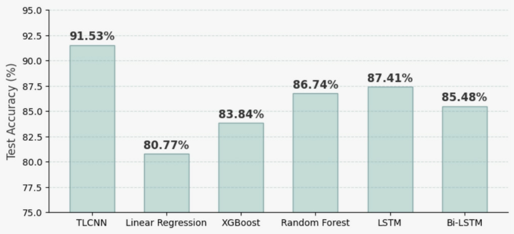
Fig.9.Test accuracy comparison of TLCNN with ML and RNN algorithms.

Furthermore,Fig.10 illustrates a side-by-side comparison of Mean Squared Error (MSE) and Mean Absolute Error (MAE) across six different models,highlighting the predictive reliability of TLCNN.The proposed model demonstrates the lowest MSE (0.0542) and MAE(0.1290),showcasing its ability to minimize both small and large prediction deviations.LSTM and Bi-LSTM also outperform traditional ML models in error minimization,with MSE/MAE scores of 0.0872/0.2355 and 0.1341/0.2923 respectively.However,their performance does not surpass that of TLCNN,which is better at capturing fine-grained patterns within high-dimensional tabular data.These results further support the model’s robustness in producing precise forecasts while maintaining computational efficiency.

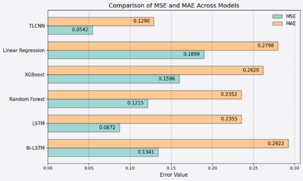
Fig.10.Comparison of MSE and MAE across four different models.

4.2 Visual iz ing TLCNN model effectiveness

To fur ther investigate the effectiveness of the TLCNN model,various visual representations of training dynamics and prediction accuracy are analyzed. Fig.11 illustrates the training and validation loss curves,providing insights into the convergence behavior of the model.The smooth decline in loss values indicates stable learning and reduced risk of overfitting.This be havior demonstrates that TLCNN maintains consistent gradient updates,reflecting the optimizer’s effectiveness (Adam) and the model’s ability to generalize well without oscillations or divergence—a common issue in deeper CNNs or improperly tuned networks.Comparatively,the traditional machine learning models lack such a direct way to monitor convergence and optimization during training.

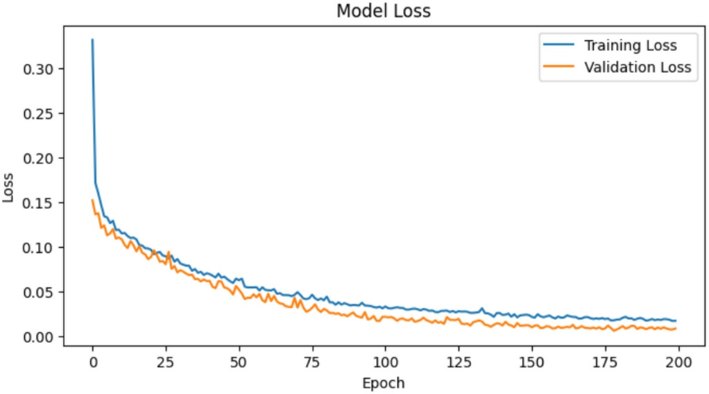
Fig.11.Training loss and validation loss curve.

Fig.12 presents the training and validation MAE curves,demonstrating the model’s ability to minimize absolute errors over successive epochs.The consistency between training and validation curves suggests that TLCNN does not suffer from significant overfitting,ensuring reliable predictions.Notably,the minimal gap between training and validation MAE across epochs highlights strong model generalization,especi ally important in regression tasks on non-image,structured datasets like BanE-16.The gradual decline in MAE rather than a sharp drop followed by fluctuation suggests that the model’s architecture and hyperparameters are well-aligned for learning temporal and contextual relationships embedded in the tabular features.

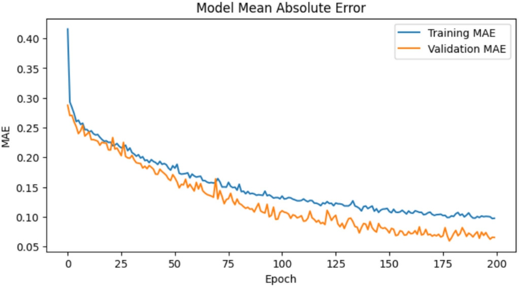
Fig.12.Training MAE and validation MAE curve.

Additionally,a direct comparison between actual and predicted values is visualized to evaluate the model’s predictive accuracy in real-world scenario s.The plotted results illustrate the strong alignment between predicted energy demand and actual observed values,reinforcing TLCNN’s robustness in capturing complex data patterns.InFig.13,the tight overlap between the predicted (blue)and actual (red) lines demonstrates the model’s responsiveness to short-term variations and its stability across fluctuating demand points.The relatively small residuals across multiple time points confirm that the model avoids high variance behavior,unlike many overfit neural networks.This alignment validates TLCNN’s capacity not only for high average accuracy but also for capturing the temporal irregularities common in energy consumption trends.The TLCNN model’s inference time was measured on the test set consisting of 779 samples.The total inference time was approximately 212 ms,resulting in an average per-sample inference time of 0.272 ms.

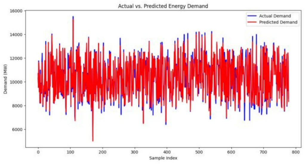
Fig.13.Visualization of real and forecasted energy demand over sample timepoints.

Fig.14 reveals how batch size,activation functions,optimizers,learning rate,and number of epochs influence TLCNN’s performance.For instance,using ReLU activation and Adam optimizer yielded the lowest MSE and MAE,confirming their suitability in shallow CNN architectures processing non-visual data.The trends also indicate that overly large batch sizes or aggressive optimizers(like SGD) lead to higher error rates,reflecting the need for balanced training dynamics in lightweight architectures.

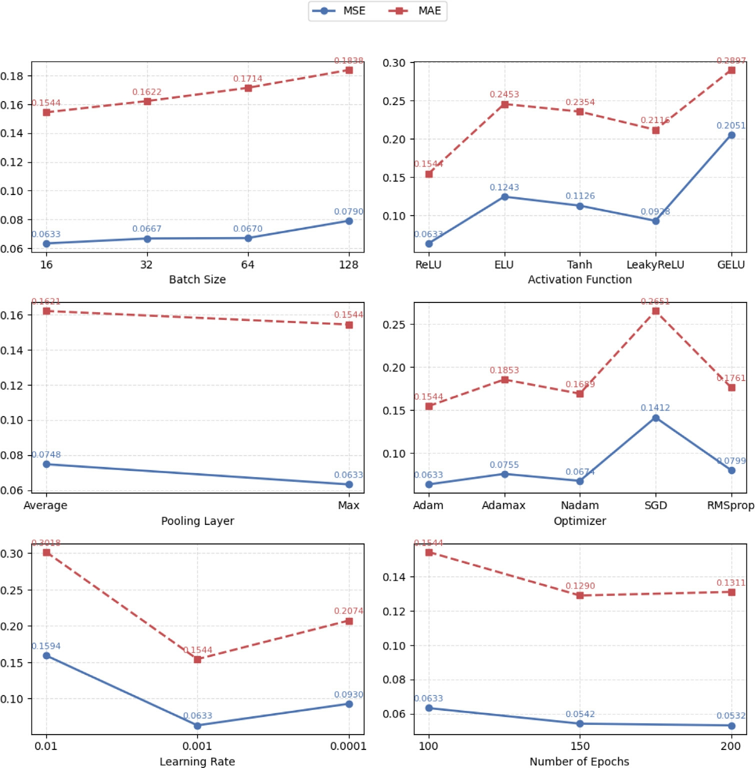
Fig.14.Plot trends for MSE and MAE under different configurations of TLCNN.

4.3 Ablation study

An ablation study is conducted by tuning various hyperparameters to enhance the performance of the proposed TLCNN model.The study comprises six experiments,where the optimal hyperparameter for each experiment is selected based on the highest accuracy,lowest Mean Squared Error (MSE),and lowest Mean Absolute Error (MAE).The detailed results are presentedin Table 4.Initially,the number of epochs is fixed at 100.With this configuration,Study 1 explores the impact of different batch sizes.A batch size of 16 yields the highest accuracy (88.19%) while also achieving the lowest MSE(0.0633) and MAE (0.1544).Building on this,Study2 investigates the effect of activation functions.Among the tested functions,ReLU delivers the best performance,maintaining the previously achieved highest accuracy and lowest error metrics.In Study 3,different pooling layers are examined.MaxPooling outperforms AveragePooling across all metr ics,reaffirming the highest accuracy(88.19%) and lowest MSE (0.0633) and MAE (0.1544).

Table 4 The result of the ablation study of TLCNN.

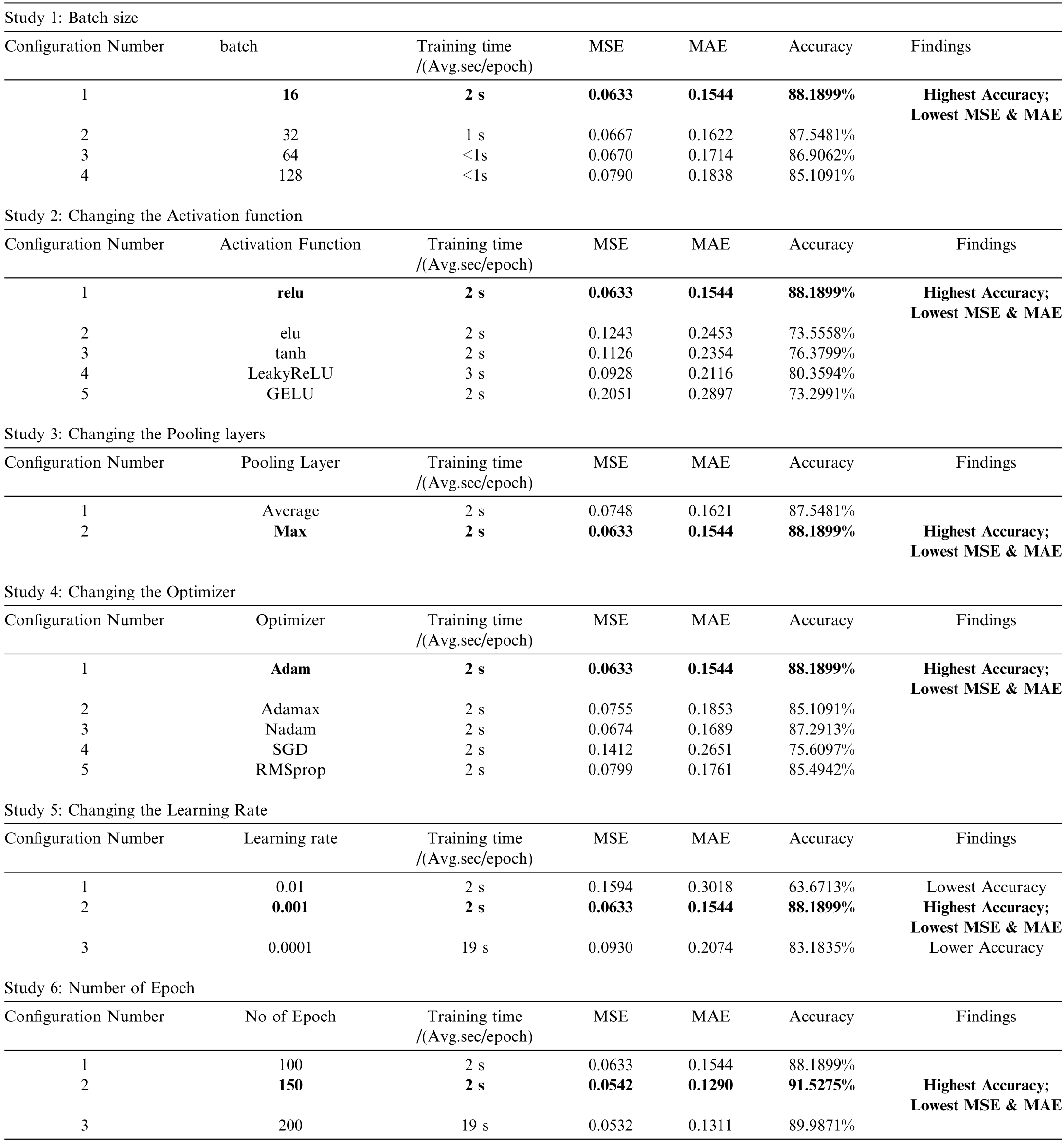
Study 4 evaluates various optimizers,including Adam,Adamax,Nadam,SGD,and RMSprop.Adam emerges asthe best optimizer,preserving the previously obtained optimal performance.Next,Study 5 explores different learning rates.An optimal learning rate of 0.001 is identified,which is used for subsequent experiments.Finally,Study 6 investigates the effect of varying the numberof epochs (100,150,and 200) while keeping other hyperparameters constant.The results indicate that training for 150 epochs achieves the highest accuracy (91.53%),along with the lowest MSE (0.0542) and MAE (0.1290).While increasing the epochs to 200 slightly reduces MSE(0.0532),it results in a minor accuracy drop (89.99%)and an increase in MAE(0.1311).Based on these findings,150 epochs are selected as the optimal training duration for TLCNN.Based on these findings,the final TLCNN configuration consists of a batch size of 16,ReLU activation,MaxPooling,Adam optimizer,a learning rateof 0.001,and 150 epochs,ensuring optimal performance.

4.4 Summary of findings

The empirical analysis demonstrates that TLCNN consistently outperforms traditional machine learning and deep learning models in terms of accuracy and error minimization.Unlike Linear Regression,which struggles with capturing non-linear relationships,TLCNN effectively extracts meaningful patterns,resulting in superior generalization.XGBoost,while powerful in certain applications,exhibits overfitting tendencies,leading to reduced test accuracy despite strong training performance.Random Forest,although competitive in accuracy,does not minimize errors as effectively as TLCNN.LSTM and Bi-LSTM offer better generalization than ML baselines but fail to achieve the low MSE and MAE demonstrated by TLCNN,confirming the superior performance of our proposed method.

The visualizations support these findings,showcasing TLCNN’s stability during training and its ability to maintain low MSE and MAE values under different conditions.The plotted actual vs.predicted values further confirm that TLCNN provides reliable energy demand forecasts,making it a suitable model for high-dimensional and complex datasets.

Overall,the results substantiate the effectivenessof TLCNN as an optimized and efficient approach for energy demand prediction.By leveraging deep learning capabilities,the model successfully overco mes the limitationsof conventional machine learning and deep learning methods,offering a reliable solution for predictive modeling in tabular datasets.

5 Discussion

The findings of this study demonstrate that the proposed Tabular Lightweight Convolutional Neural Network (TLCNN) outperforms conventional machine learning models,such as Linear Regression,XGBoost,and Random Forest,and deep learning models-LSTM,Bi-LSTM in energy demand forecasting.TLCNN effi-ciently captures complex,non-linear dependencies in tabular data,which traditional models often fail to recognize,leading to enhanced generalization and reduced prediction errors.Unlike Linear Regression,which struggles with intricate,non-linear relationships,TLCNN identifies these hidden patterns,improving predictive accuracy.While XGBoost is highly effective in structured data modeling,it is prone to overfitting,limiting its generalization capabilities.Similarly,Random Forest,though competitive,does not minimize Mean Squared Error (MSE) and Mean Absolute Error (MAE) as effectively as TLCNN.The experimental results further validate TLCNN’s stability,with consistently lower MSE and MAE values across multiple evaluations,confirming its reliability in energy demand forecasting.One of the key advantagesof TLCNN is its lightweight architecture,which addresses computational inefficiencies commonly associated with deep learning models for tabular data.Unlike traditional CNN-based approaches that require data transformation into image-like formats,TLCNN operates directly on tabular data,enhancing both efficiency and predictive performance.This direct processing makes TLCNN well-suited for real-time energy forecasting systems where computational resources are constrained.The integrationof TLCNN in energy demand forecasting holds significant societal and environmental implications.Accurate demand prediction optimizes resource distribution,preventing power shortages and reducing supply disruptions.Improved forecasting also helps energy providers optimize generation,lowering costs and ensuring affordable pricing.TLCNN’s efficiency makes it suitable for both large-scale and small-scale energy management,benefiting regions with limited infrastructure.Environmentally,precise forecasting minimizes energy waste,improves grid management,and reduces reliance on fossil fuels,leading to lower carbon emissions.It also supports renewable energy integration by adapting to demand fluctuations,promoting sustainability.By enhancing smart grid efficiency,TLCNN contributes to environmentally friendly policies.Despite its advantages,this study has limitations.The BanE-16 dataset,while comprehensive,remains relatively small.Future research should explore TLCNN’s performance on larger datasets to assess scalability.Additionally,while this study focuses on energy demand,TLCNN could be applied in healthcare,finance,and climate modeling.Exploring hybrid architectures,suchas CNN-Transformer models,may further improve accuracy.In summary,TLCNN presents an efficient,accurate,and computationally lightweight alternative to traditional machine learning models.Its ability to extract meaningful patterns,minimize errors,and operate efficiently makesit a valuable tool for real-time forecasting,advancing energy informatics and sustainable energy planning.In comparison to existing CNN-based approaches in the literature,the proposed TLCNN model demonstrates significantly enhanced performance.For instance,A study [37]of CNN based Energy demand forcasting reports a minimum MSE of 0.50 on their test set,whereas our TLCNN model achieves a notably lower MSE of 0.0542.This substantial reduction in error indicates the effectiveness of our lightweight CNN architecture in capturing complex patterns within tabular data without the need for optimizationbased tuning or image transformations.Such improvement emphasizes the value of TLCNN as a more efficient and accurate approach for energy demand forecasting,particularly in real-world settings where high prediction accuracy and low error tolerance are critical.

6 Conclusion

This study introduced TLCNN,a novel lightweight CNN model designed to predict electricity supply and demand directly from tabular data without the need for image transformation.Unlike traditional approaches that rely on manually engineered features or data transformations,TLCNN efficiently captures spatial dependencies intabular datasets,enhancing forecasting accuracy while maintaining computational efficiency.Extensive data preprocessing,including feature selection,standard scaling,and reshaping,was performed to ensure the dataset’s compatibility with CNNs.TLCNN was compared against multiple machine learning and deep learning models to validate its effectiveness,demonstrating superior performance in energy demand prediction.The key contribution ofthis research lies in bridging the gap between CNNs and tabular data processing,offering a more adaptable and scalable solution for energy forecasting.By implementing CNN-based feature extraction without requiring image conversion,TLCNN presents a computationally efficient alternative to traditional methods,making it highly applicable for real-time energy management systems.However,this study is not without limitations.The dataset used,while representative,is relatively small in scale,which may affect the model’s generalizability to larger or more diverse regions.Additionally,the evaluation is limited to energy demand data from a specific geographic context,and model performance may vary across different sectors orcountries.Moreover,although TLCNN reduces computational overhead,deep learning models still require higher training time compared to some lightweight ML models.Future research can address these limitations by leveraging larger-scale multi-regional datasets,experimenting with cross-domain applications(such as in healthcare or transportation),and optimizing the architecture for even lower resource consumption.In conclusion,by addressing the challenges associated with CNN-based tabular data processing,this study contributes to the advancement of AI-driven energy management systems,paving the way for more accurate, style="font-size: 1em; text-align: justify; text-indent: 2em; line-height: 1.8em; margin: 0.5em 0em;">Declaration of Generative AI and AI-assisted technologies inthe writing process

The authos improve the article’s vocabulary and readability during the writing process by utilizing the ChatGPT service.After utilizing this ChatGPT service,reviewing and editing it as necessary,the authors take full responsibility for the publication’s content.

CRediT authorship contribution statement

Nazmul Huda Badhon: Validation,Visualization,Data curation,Methodology,Writing– original draft,Formal analysis.Imrus Salehin: Writing– review &editing,Data curation,Formal analysis,Writing– original draft,Conceptualization,Supervision.Md Tomal Ahmed Sajib: Writing– original draft,Methodology,Visualization,Validation. Md Sakibul Hassan Rifat: Writing– original draft,Methodology,Visualization,Software. S.M.Noman: Writing– original draft,Data curation,Methodology,Formal analysis.Nazmun Nessa Moon: Supervision,Writing– review &editing.

Declaration of competing interest

The authors state that any known competing financial interests or personal relationships could have influenced none of the work described in this study.

Data availabil ity

Publicly available datasets were analyzed in this study.These data can be found here (accessed on 3 April 2024):-BanE-16: https://doi.org/10.17632/3brbjpt39s.2.Access link: https://data.mendeley.com/datasets/3brbjpt39s/2.

References

[1]W.G.Santika,M.Anisuzzaman,Y.Simsek,et al.,Implications of the sustainable development goals on national energy demand:the case of Indonesia,Energy 196 (2020) 117100.

[2]E.Ridha,L.Nolting,A.Praktiknjo,Complexity profiles: a largescale review of energy system models in terms of complexity,Energ.Strat.Rev.30 (2020) 100515.

[3]S.Pfenninger,A.Hawkes,J.Keirstead,Energy systems modeling for twenty-first century energy challenges,Renew.Sustain.Energy Rev.33 (2014) 74–86.

[4]L.Kotzur,L.Nolting,M.Hoffmann,et al.,A modeler’s guide to handle complexity in energy systems optimization,Adv.Appl.Energy 4 (2021) 100063.

[5]C.S.E.Bale,L.Varga,T.J.Foxon,Energy and complexity: new ways forward,Appl.Energy 138 (2015) 150–159.

[6]A.Cherp,J.Jewell,A.Goldthau,Governing global energy:sys tems,transitions,complexity,Global Pol.2 (1) (2011) 75–88.

[7]A.Agga,A.Abbou,M.Labbadi,et al.,CNN-LSTM: an efficient hybrid deep learning architecture for predicting short-term photovoltaic power production,Electr.Pow.Syst.Res.208(2022) 107908.

[8]S.A.Adewuyi,S.G.Aina,A.I.Oluwaranti,A deep learning model for electricity demand forecasting based on a tropical data,Appl.Comput.Sci.16 (1) (2020) 5–17.

[9]R.Wazirali,E.Yaghoubi,M.S.S.Abujazar,et al.,State-of-the-art review on energy and load forecasting in microgrids using artificial neural networks,machine learning,and deep learning techniques,Electr.Pow.Syst.Res.225 (2023) 109792.

[10]K.Amasyali,N.M.El-Gohary,A review of name="ref11" style="font-size: 1em; text-align: justify; text-indent: 2em; line-height: 1.8em; margin: 0.5em 0em;">[11]M.Frikha,K.Taouil,A.Fakhfakh,et al.,Limitation of deeplearning algorithm for prediction of power consumption,in:Proceedings of The 8th International Conference on Time Series and Forecasti ng,2022,p.26.

[12]M.Khalil,A.S.McGough,Z.Pourmirza,et al.,Machine learning,deep learning and statistical analysis for forecasting building energy consumption: a systematic review,Eng.Appl.Artif.Intel.115 (2022) 105287.

[13]J.H.Qin,W.Y.Pan,X.Y.Xiang,et al.,A biological image classification method based on improved CNN,Eco.Inform.58(2020) 101093.

[14]M.T.Sarker,M.Jaber Alam,G.Ramasamy,et al.,Energy demand forecasting of remote areas using linear regression and inverse matrix analysis [J],Int.J.Electr.Comput.Eng.(IJECE) 14 (1)(2024) 129.

[15]A.A.Elngar et al.,Image classification based on CNN:a survey,J.Cybersecur.Informat.Manag.(2021),PP.18-PP.50.

[16]F.Sultana,A.Sufian,P.Dutta,Advancements in image classification using convolutional neural network,in: Proceedings of 2018 Fourth International Conferen ce on Research in Computational Intelligence and Communication Networks(ICRCICN),IEEE,Kolkata,India,2018,pp.122–129.

[17]I.Salehin,S.M.Noman,M.M.Hasan,Electricity energy dataset“BanE-16”: Analysis of peak energy demand with environmental variables for machine learning forecasting,Data Brief 52 (2024)109967.

[18]T.Manojpraphakar,Energy demand prediction using linear regression,in: Proceedings of International Conference on Artificial Intelligence,Smart Grid and Smart City Applications:AISGSC 2019,2020,pp.407–417.

[19]G.Ciulla,A.D’Amico,Building energy performance forecasting:a multiple linear regression approach,Appl.Energy 253 (2019)113500.

[20]T.Z.Zhang,X.N.Zhang,O.Rubasinghe,et al.,Long-term energy and peak power demand forecasting based on sequential-XGBoost,IEEE Trans.Power Syst.39 (2) (2024) 3088–3104.

[21]R.A.Abbasi,N.Javaid,M.N.J.Ghuman,et al.,Artificial iIntelligence and network applications,Proc.Workshops 33rd Int.Conf.Adv.Informat.Net.Appl.(WAINA-2019) 33 (2019)1120–1131.

[22]H.Rathore,H.K.Meena,P.Jain,Prediction of EV energy consumption using random forest and XGBoost,in: Proceedings of 2023 International Conference on Power Electronics and Energy(ICPEE),IEEE,Bhubaneswar,India,2023,pp.1–6.

[23]Z.Y.Wang,Y.R.Wang,R.C.Zeng,et al.,Random forest based hourly building energy prediction,Energ.Build.171 (2018) 11–25.

[24]L.Cáceres,J.I.Merino,N.Díaz-Dí az,A computational intelligence approach to predict energy demand using random forest in a cloudera cluster,Appl.Sci.11 (18) (2021) 8635.

[25]Y.T.Zhu,T.Brettin,F.F.Xia,et al.,Publisher Correction:Converting tabular data into images for deep learning with convolutional neural networks,Sci.Rep.11 (2021) 14036.

[26]B.S.Bharath,J.Bollineni,S.P.Mandala,et al.,Anatomizationof neural networks based models for semantic analysis of tabular dataset,in,in: Proceedings of 2024 IEEE 9th International Conference for Convergence in Technology (I2CT),IEEE,Pune,India,2024,pp.1–8.

[27]T.K.Vyas,Deep learning with tabular data: a self-supervised approach.arXiv preprint arXiv:2401.15238.(2024).

[28]V.Jain,M.Goel,K.Shah,Deep learning on small tabular dataset:using transfer learning and image classification,in: Proceedingsof International Conference on Artificial Intelligence and Speech Technology,2021,pp.555–568.

[29]M.I.Iqbal,M.S.H.Mukta,A.R.Hasan,et al.,A dynamic weighted tabular method for convolutional neural networks,IEEE Access10(2022) 134183–134198.

[30]A.Islam,M.T.Ahmed,M.A.H.Mondal,et al.,A snapshot of coalfired power generation in Bangladesh: a demand–supply outlook,Nat.Res.Forum 45 (2) (2021) 157–182.

[31]A.Islam,M.B.Hossain,M.A.H.Mondal,et al.,Energy challenges for a clean environment: Bangladesh’s experience,Energy Rep.7(2021) 3373–3389.

[32]T.Ahmad,H.C.Zhang,B.Yan,A review on renewable energy and electricity requirement forecasting models for smart grid and buildings,Sustain.Cities Soc.55 (2020) 102052.

[33]S.Aslam,H.Herodotou,S.M.Mohsin,et al.,A survey on deep learning methodsfor power load and renewable energyforecasting in smart microgrids,Renew.Sustain.Energy Rev.144(2021)110992.

[34]N.A.Mohammed,Modelling of unsuppres sed electrical demand forecasting in Iraq for long term,Energy 162 (2018) 354–363.

[35]M.Qureshi,M.Ahmad Arbab,S.U.Rehman,Deep learning-based forecasting of electricity consumption,Sci.Rep.14 (2024) 6489.

[36]X.J.Luo,L.O.Oyedele,Forecasting building energy consumption:Adaptive long-short term memory neural networks drivenby genetic algorith,Adv.Eng.Inf.50 (2021) 101357.

[37]H.H.Hu,S.F.Gong,B.Taheri,Energy demand forecasting using convolutional neural network and modified war strategy optimization algorithm,Heliyon 10 (6) (2024) e27353.

[38]T.Le,M.Vo,B.Vo,et al.,Improving electric energy consumption prediction using CNN and Bi-LSTM,Appl.Sci.9(20)(2019)4237.

[39]G.Fotis,N.Sijakovic,M.Zarkovic,et al.,Forecasting wind and solar energy production in the Greek power system using ANN models,Wseas Trans.Power Syst.18 (2023) 373–391.

[40]S.H.Almuhaini,N.Sultana,Forecasting long-term electricity consumption in Saudi Arabia based on statistical and machine learning algorithms to enhance electric power supply management,Energies 16 (4) (2023) 2035.

[41]A.A.Pierre,S.A.Akim,A.K.Semenyo,et al.,Peak electrical energy consumption prediction by ARIMA,LSTM,GRU,ARIMA-LSTM and ARIMA-GRU approaches,Energies 16 (12)(2023) 4739.

[42]A.Hameedah,J.Berri,Transforming tabular data into images via enhanced spatial relationships for cnn processing,Sci.Rep.15(2025).https://api.semanticscholar.org/CorpusID:278705313.

[43]T.Tsiligkaridis,A.Tsiligkaridis,Diverse Gaussian noise consistency regularization for robustness and uncertainty calibration,in: Proceedings of 2023 International Joint Conference on Neural Networks (IJCNN),IEEE,Gold Coast,Australia,2023,pp.1–8.

[44]F.Pedregosa,(2024) Standardscaler.https://scikit-learn.org/stable/modules/generated/sklearn.preprocessing.StandardScaler.html,2011.Accessed: 2024-09-12.

[45]Q.S.Wen,L.Sun,X.M.Song,et al.,Time series data augmentation for deep learning: A survey,Int.Joint Conf.Artif.Intell.(2021).

[46]M.Arslan,M.Guzel,M.Demirci,et al.,SMOTE and Gaussian noise based sensor data augmentation,in: 2019 4th International Conference on Computer Science and Engineering (UBMK),IEEE,Samsun,Turkey,2019,pp.1–5.

[47]A.EL Bilali,A.Taleb,M.A.Bahlaoui,et al.,An integrated approach based on Gaussian noises-based data augmentation method and AdaBoost model to predict faecal coliforms in rivers with small dataset,J.Hydrol.599 (2021) 126510.

[48]C.Khosla,B.S.Saini,Enhancing performance of deep learning models with different data augmentation techniques: a survey,in:Proceedings of 2020 International Conference on Intelligent Engineering and Management (ICIEM),IEEE,London,United Kingdom,2020,pp.79–85.

[49]J.Wu,Introduction to convolutional neural networks,National Key Lab for Novel Software Technology,Nanjing University.China,2017,p.495,5 (23).

[50]F.Alrasheedi,X.Zhong,P.C.Huang,Padding module: Learning the padding in deep neural networks,IEEE Access 11(2023)7348–7357.

[51]J.Nagi,F.Ducatelle,G.A.Di Caro,et al.,Max-pooling convolutional neural networks for vision-based hand gesture recognition,in: Proceedings of 2011 IEEE International Conference on Signal and Image Processing Applications(ICSIPA),IEEE,Kuala Lumpur,Malaysia,2011,pp.342–347.

[52]T.Q.Chen,C.Guestrin,XGBoost: A scalable tree boosting system,in: Proceedings of the 22nd ACM SIGKDD InternationalConference on Knowledge Discovery and Data Mining,ACM,San Francisco California USA,2016,pp.785–794.

Received 25 October 2024;revised 22 May 2025;accepted 8 July 2025

Peer review under the responsibility of Global Energy Interconnection Group Co.Ltd.

* Corresponding author.

E-mail address:imrus15-8978@diu.edu.bd (I.Salehin).1 Authors Imrus Salehin and Nazmul Huda Badhon contributed equally to this work.

https://doi.org/10.1016/j.gloei.2025.07.005

2096-5117/© 2025 Global Energy Interconnection Group Co.Ltd.Publishing services by Elsevier B.V.on behalf of KeAi Communications Co.Ltd.This is an open access article under the CC BY-NC-ND license(http://creativecommons.org/licenses/by-nc-nd/4.0/).

Nazmul Huda Badhon is a deep learning researcher who holds a Bachelor of Science degree in Computer Science and Engineering from Daffodil International University,Bangladesh (2025).He completed a semester in Computer Engineering at Dongseo University,South Korea,under the fully funded Global Korea Scholarship(GKS)exchange program in 2023,gaining deeper expertise in artificial intelligence.His research interests include machine learning,deep learning,convolutional neural networks,and their applications in med ical AI.He has authored multiple peer-reviewed publications with Els evier,Wiley,and Taylor&Francis,and has been actively involved in rese arch and peer reviewactivities.He received the ’Researcher of the Year 2024’ award from the Division of Research,Daffodil International University.