0 Introduction

The widespread development and application of fossil fuels have become important factors in maintaining social operations over the recent centuries [1,2].Simultaneously,the energy-demand gap among countries is constantly expanding.Conventional power supplies rely on significant amounts of conventional fossil resources, which are both limited and nonrenewable [3,4].Additionally, excessive exploitation of fossil fuels has caused severe and even permanent damage to land,water sources,and ecosystems,thus resulting in numerous environmental issues with longterm and irreversible impacts [5,6].Hence, countries worldwide are actively promoting sustainable, diversified,and environmentally friendly renewable-energy development [7].

In this context, solar energy, which is one of the most representative clean and renewable energy sources, has been extensively utilized in various industries worldwide owing to its abundant reserve, low noise, and zero emission [8-10].During photovoltaic (PV) power generation,the output characteristics of PV models are related not only to the external temperature and solar irradiance but also to several critical operation parameters inside the PV cell [11-13].However, the internal operating parameters of PV models are not provided by the manufacturer and change over time.Therefore, these parameters inside a PV cell must be identified to achieve more accurate PV-cell modeling.Currently, three mathematical PV cell models are widely recognized and applied, namely, the single-diode model (SDM), double-diode model (DDM),and three-diode model (TDM).Because of their greater number of unknown parameters, the DDM and TDM are more complex and cost more for parameter identification as compared with the SDM; however, they provide more details regarding the operation characteristics of PV models [14,15].

As the parameter identification of PV cells is a nonlinear function-optimization problem with multiple variables and peaks,the optimal solutions cannot be easily obtained using analytical methods and conventional optimization algorithms.Nonetheless,metaheuristic algorithms(MhAs)can solve this problem owing to their advantages, such as high convergence speed and non-requirement for precise system models.As shown in [16-19], the parameters of various batteries are typically identified using MhAs, and some studies improved heuristic algorithms by adding certain mechanisms or strategies.In recent years, the parameter identification of PV models has been investigated extensively.For example, the authors of [20] proposed an iterative identification algorithm based on multiple innovation gradients that can identify unknown parameters easily and effectively.However, they did not fully investigate the effects of dataset noise and insufficient data on the accuracy of recognition results.The authors of[21]developed a PV model parameter-identification strategy based on a differential evolution algorithm that involves different evolutionary stages and exhibits favorable global optimizability and rapid convergence.However,this strategy requires optimization in terms of computational complexity and runtime.The authors of [22] designed an improved adaptive particle swarm optimization algorithm that balances the search relationship between global and local extrema by introducing asynchronous learning factors, thereby improving the accuracy of parameter identification.However, this algorithm may be limited when noisy data are involved.The authors of [23] proposed an MhA that combines style="font-size: 1em; text-align: justify; text-indent: 2em; line-height: 1.8em; margin: 0.5em 0em;">In summary, previous studies primarily used MhAs and their improved variants for PV cell parameter identification to improve the accuracy and speed of parameter identification.However, almost all previous studies have overlooked the important fact that not only is the external parameter-identification design important, but also the measurement dataset used directly affects the parameter-extraction performance.The dataset has some inherent defects, such as noisy data and insufficient data samples, which reduce the accuracy of the recognition results.Therefore, this study aims to address these issues and improve the accuracy and efficiency of parameter identification in PV models.Specifically, this study employs a Bayesian neural network (BNN) as a datapreprocessing tool and artificial ecosystem optimization(AEO) as an optimization algorithm for PV cell parameter extraction.The BNN can prevent overfitting, improve prediction flexibility, and provide uncertainty estimation,whereas the AEO offers high global-search ability, convergence speed, and adaptability.In detail, the BNN is applied in the first stage of data preprocessing to filter noisy data and enrich the dataset based on data prediction, which can compensate for the adverse effect on the identification results caused by insufficient datasets and noisy data.Subsequently, AEO is performed for unknown-parameter identification based on the processed datasets.The simulation results show that after data processing, both the identification accuracy and convergence improved.

The main contributions of this study are as follows:

1) Three commonly applied PV cell models and one PV module are established, and 10 different MhAs for parameter identification for all three models are discussed and compared.

2) The effects of insufficient data, data loss, and noisy data on the accuracy of PV cell parameter identification are investigated.Based on the data preprocessing of a BNN to reduce noise and predict datasets,more accurate output current-voltage (I-V) and power-voltage (P-V) characteristic curves are obtained, thereby improving the accuracy.

3) Based on a comparison of the simulation results obtained from 10 MhAs, the AEO outperformed the other MhAs under both denoised and predicted data.

The remainder of this paper is organized as follows:Section 1 introduces the PV modeling performed, which primarily includes four PV models and their objective functions; Section 2 introduces the principles of the BNN and AEO, as well as the parameter-identification framework using BNN-MhAs; Section 3 primarily analyzes the simulation results under the SDM, DDM, and TDM; Section 4 discusses the research presented in this article; and Section 5 concludes the paper.

1 PV cell modeling

1.1 Mathematical modeling

The most widely used PV cell models are the SDM,DDM, and TDM.In this study, a PV module model with 36 cells connected in series was constructed.Detailed descriptions of the abovementioned four models are presented in Table 1.

1.2 Objective function

To identify the parameters of the PV model, tone must determine an objective function to estimate the difference between the measured and calculated data.In this regard,the root mean square error(RMSE)is typically selected as the objective function primarily because of its significant advantages as an objective function in parameter identification, including its unit consistency, error sensitivity,and wide application.By contrast,the mean squared error(MSE) and mean absolute error (MAE) have certain limi-tations, such as the MSE being susceptible to outliers and the MAE being less sensitive to significant errors.The abovementioned indicators are expressed as follows [29]:

Table 1
Summary of SDM, DDM, TDM, and PV module model.

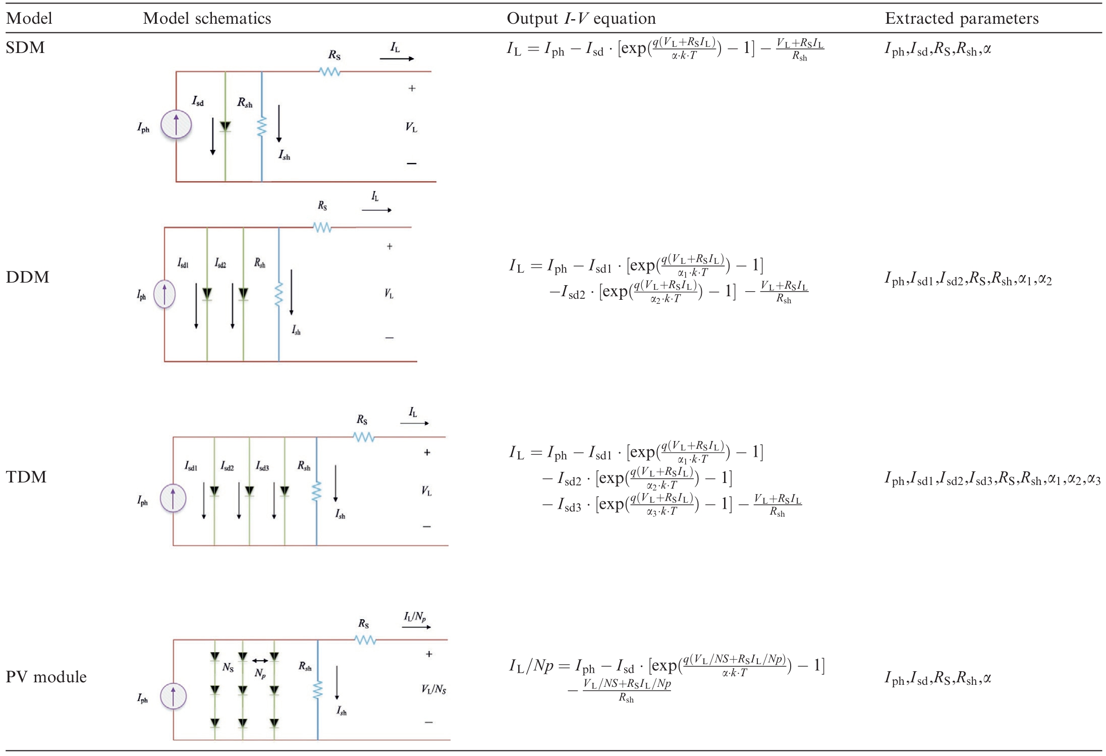
Table 2
Fitting results of various indicators.

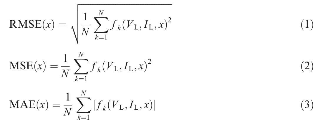
where N is the number of experimental data points;x is the solution vector, and IL and V L represent the current and voltage measurement data of the PV model, respectively.

The overlap degrees of the I-V and P-V curves, i.e.,and Rp2, respectively, are used as the evaluation criteria,which are calculated as follows:

where S is the number of input quantities;Iact and V act are the actual values of the output current and output voltage,respectively; ISC is the calculated value of the output current; and Iact is the actual average value of the output current.

Considering the SDM as an example, the MAE, MSE,and RMSE were used as indicators for parameter identification, and the obtained R2P and R2I are listed in Table 2.The symbols‘‘N”and‘‘DN”represent the result obtained using noised and denoised data, respectively.Meanwhile,the symbols ‘‘O” and ‘‘P” represent the original and predicted data,respectively.The results shows that the RMSE has the best-fitting effect for various data types.

The objective functions of the three PV models can be expressed as follows [30]:

1) SDM

2) DDM

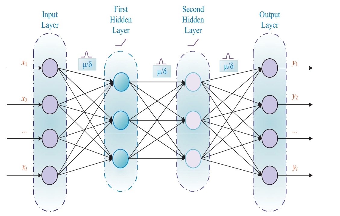
Fig.1.BNN structure diagram.

3) TDM

4) PV module model

2 PV cell parameter-identification design

2.1 Principle of BNN

The BNN considers weights to follow the mean value μ and variance δ.The Gaussian distribution follows a different distribution for each weight, and BNNs optimize the mean and variance of the weights.A diagram of the BNN structure is shown in Fig.1.

In Bayesian methods,model parameters ω use the probability distribution description.First,based on prior experience, a prior distribution p（ω） is introduced to obtain possible ω values.Assuming that the experimental dataset D = {(x1, t1), (x2, t2),..., (xn, tn)} is known and applying the Bayesian theorem, the prior distribution p（ω） is updated based on [31]:

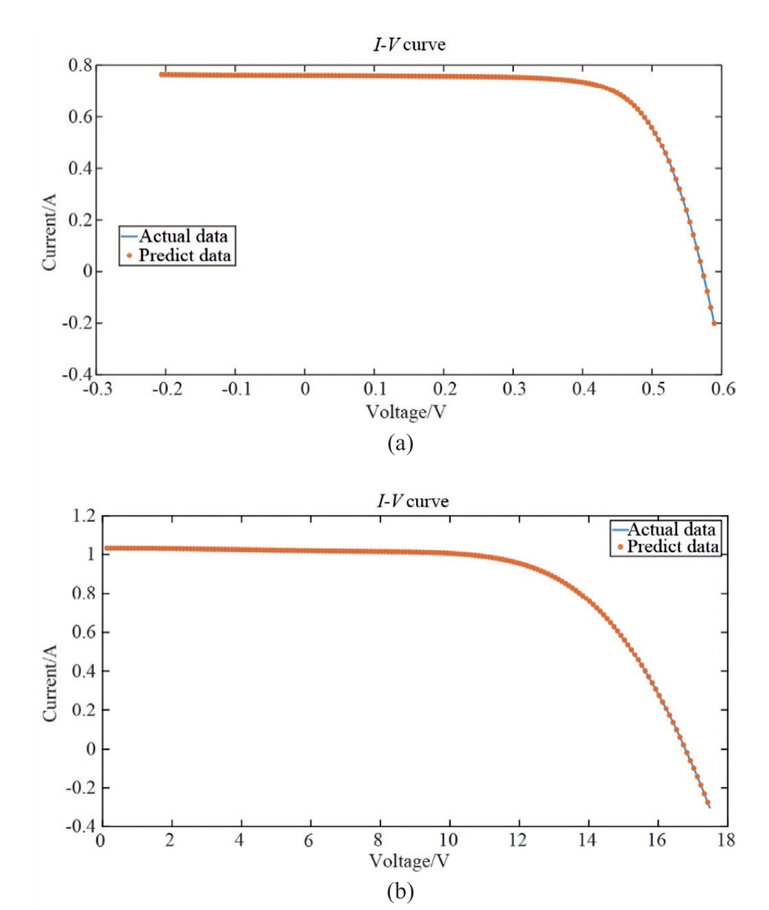
Fig.2.Result of BNN data prediction: (a) 33 C; (b) 45 C.

where xn and tn (n = 1,2,3,..., n)are the input and output data, respectively; n is the number of experimental data points; p（D|ω） is a likelihood function that contains parameters obtained from observations; p（ω|D） is the probability distribution of the posterior parameter ω of known data D, also known as the posterior distribution;p（D）is the distribution of experimental data,which serves as a normalized constant, thus ensuring that the posterior distribution is an effective probability density with a full space integral of 1.

The likelihood function p（D|ω） typically reflects the Gaussian distribution, i.e.,

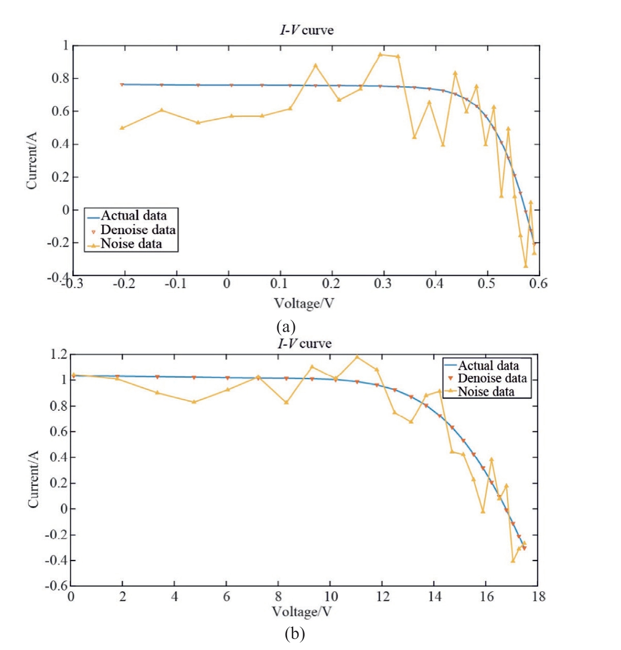
Fig.3.Result of BNN data denoising: (a) 33 C; (b) 45 C.

where Δtn is the noise error related to the nth data; ω denotes all the parameters {α，bj，cj，dij}, which are the weights and deviations of the hidden layer,and the weights and deviations of the output layer, respectively; H is the number of hidden layer neurons; and I is the number of input quantities [32].

2.2 BNN for I-V data preprocessing

The BNN constructed in this study is based on[32],and the code required approximately 3 s to process.Owing to their complex operating environments, PV models are easily affected by noise.This type of noise can affect the parameter identification of PV models, thus resulting in inaccurate final identification results.This study adopts the BNN, which further associates and reduces noise in the data.The results of BNN denoising are shown in Fig.2.

In fact, the amount of data can affect the accuracy of parameter identification.However,the current and voltage data can be insufficient and difficult to obtain.Therefore,this study trains the existing I-V data using a BNN and then performs data prediction.The prediction results obtained using the BNN are shown in Fig.3.

2.3 Principle of AEO

AEO is an emerging metaheuristic optimization algorithm that replicates the energy flow in the Earth’s ecosystem.The algorithm simulates the production,consumption, and decomposition behaviors in an ecosystem using production, consumption, and decomposition operators to solve optimization problems [33].

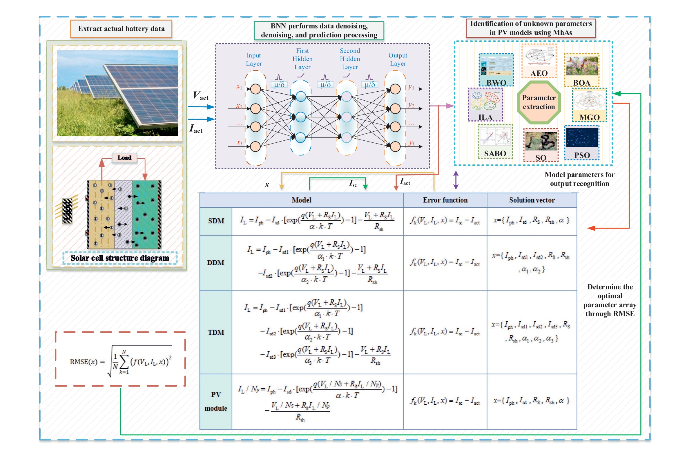
Fig.4.Schematic diagram of PV parameter identification based on BNN-MhAs.

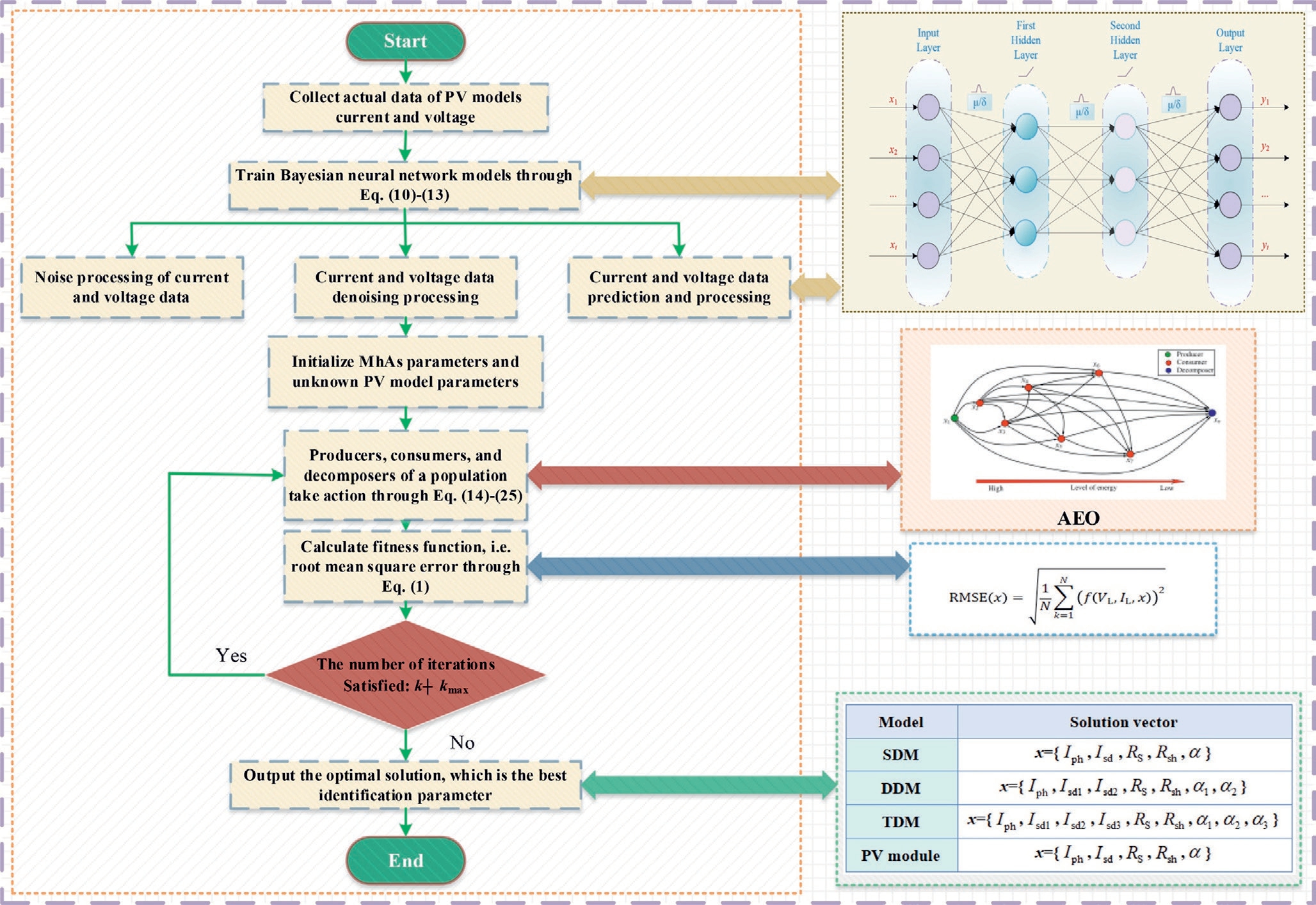
Fig.5.Intelligent parameter identification of PV cell based on BNN-AEO.

1) Production

In the AEO algorithm,the producer in the population is updated by searching for the upper and lower bounds of the space and the decomposer.The mathematical model for simulating producer behavior is established as follows:

where n is the number of individuals in a population; T is the maximum number of iterations;L and U are the lower and upper limits, respectively; r1 is a random number within the interval of [0,1]; r is a random vector within the interval of [0,1]; a is the linear weight coefficient; and xrand is the random position of an individual in the search space.

Table 3
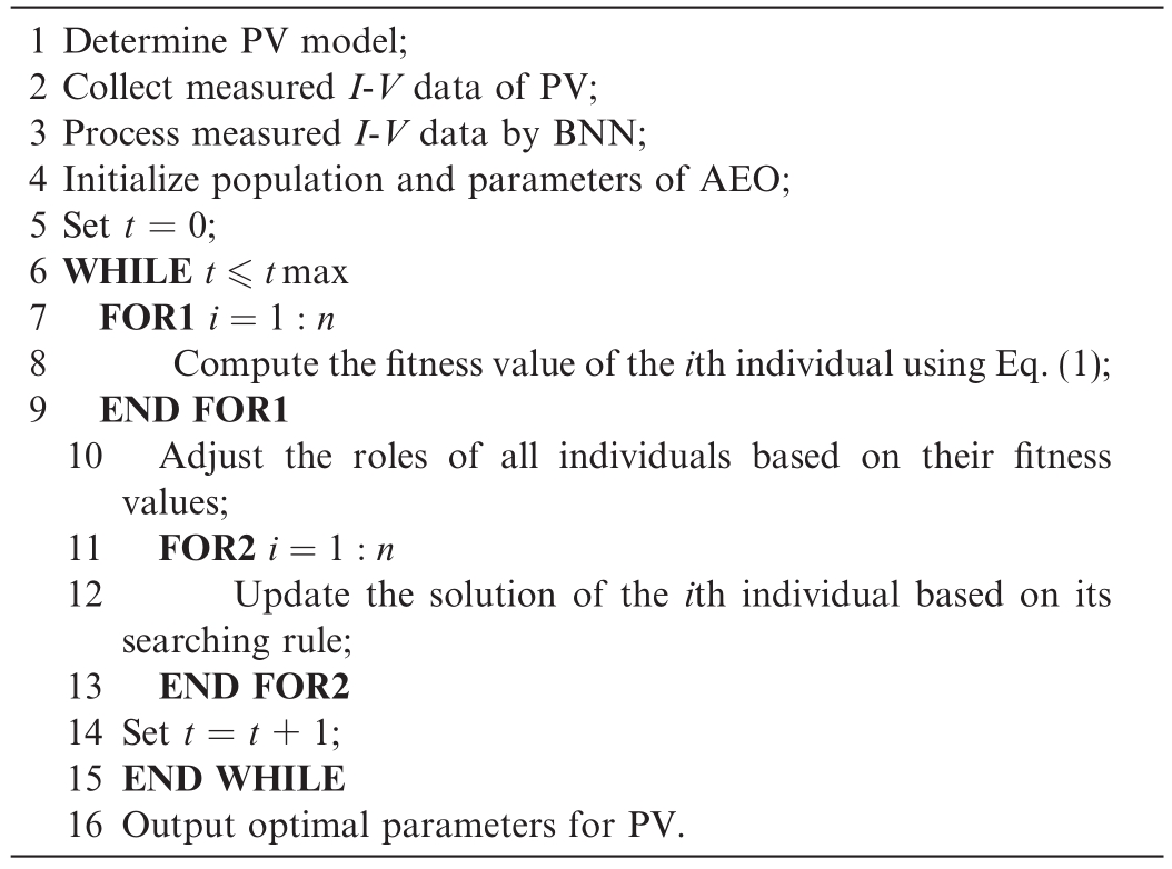
Identification steps of BNN-AEO for PV parameter extraction.

2) Consumption

After producers provide food energy, they can randomly select consumers with lower energy levels, producers, or both to obtain food energy.To facilitate this, a simple,parameter-less random walk with Levy flight characteristics is adopted, which is directly adjusted via the consumption factor, which is expressed as

where N represents a normal distribution with a mean of 0 and a standard deviation of 1.

The consumption behavior of herbivores is expressed mathematically as follows:

Table 4
V-I data under variable temperature.

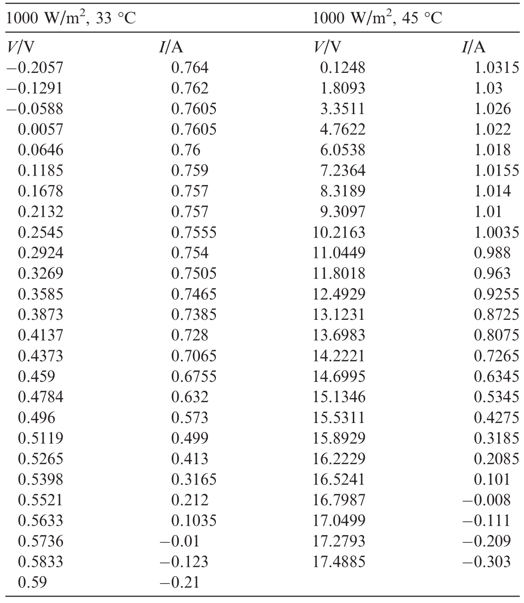
Table 5
Specifications of RTC France and PWP-201.

The consumption behavior of carnivores is expressed mathematically as follows:

The consumption behavior of omnivores is expressed mathematically as follows:

where r2 is a random number within the interval of [0,1].

3) Decomposition

Decomposers provide the necessary nutrients to the producers.The AEO algorithm allows the next position of each individual to propagate around the decomposer.The mathematical model for simulating the decomposition behavior is expressed as

Table 6
Main parameters of each MhA.

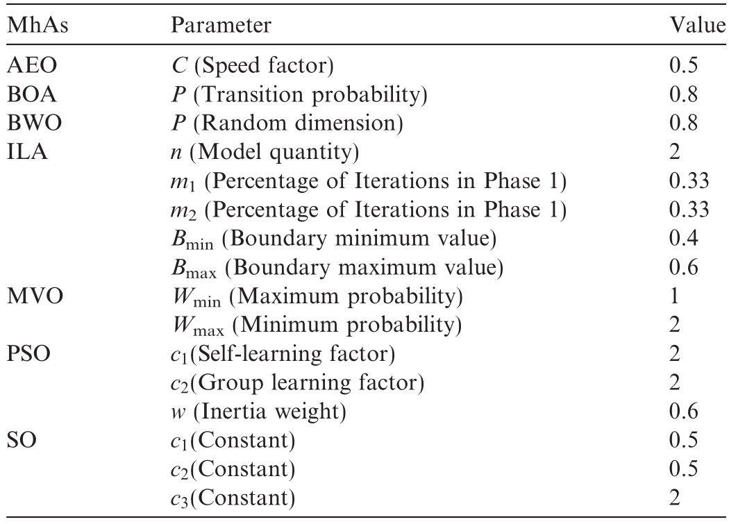
Table 7
PV model operation and MhA parameter settings.

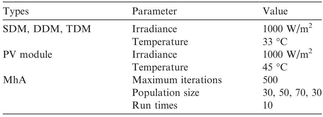
Table 8
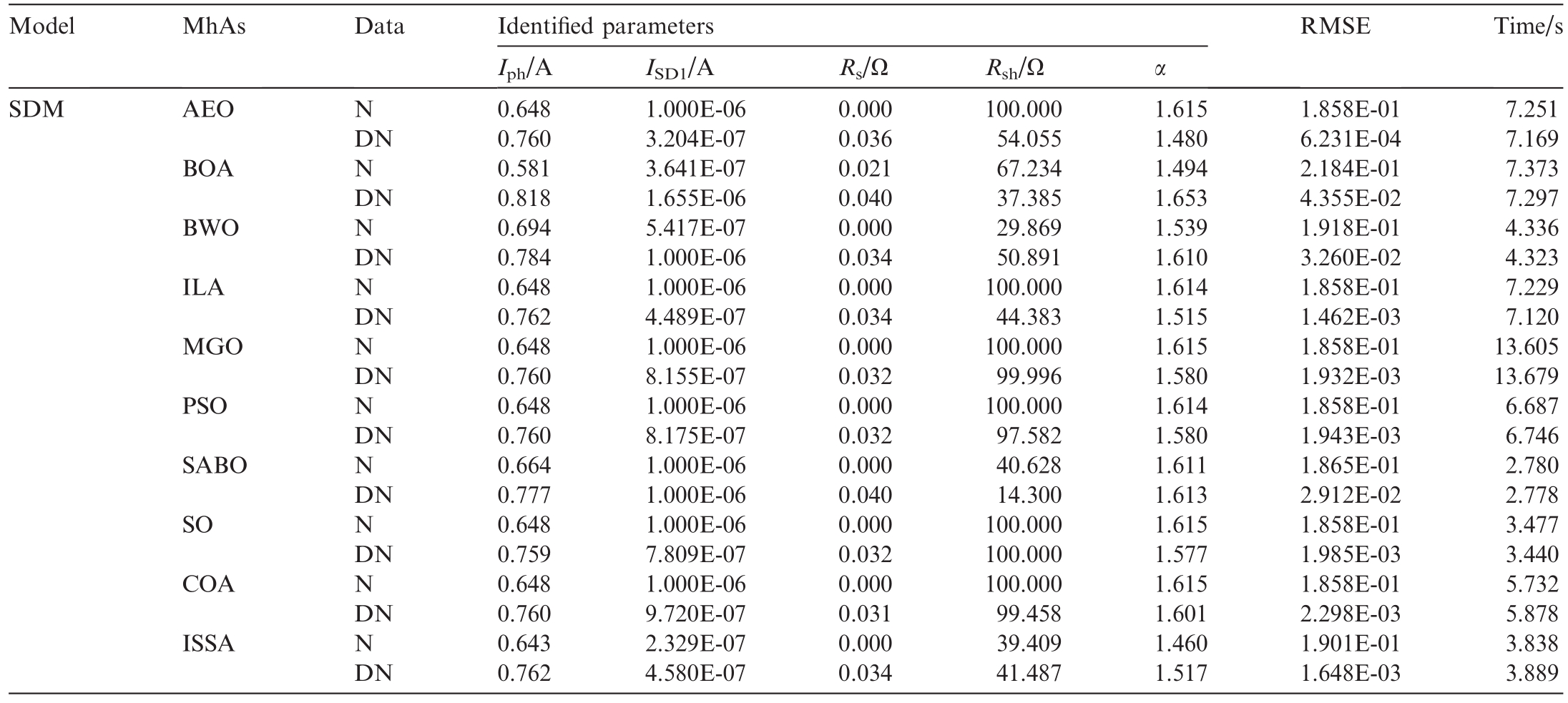
Parameter-identification results of noisy and denoised data based on 10 MhAs for SDM.

where r3 is a random number within the interval[0,1],De is the decomposition factor, and e and h are the weight coefficients.

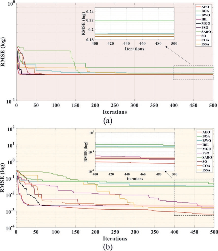
Fig.6.Convergence curves of RMSEs obtained by 10 MhAs for SDM under noisy and denoised data: (a) noisy data; (b) denoised data.

2.4 Parameter-identification process

The parameter-identification process for PV models based on BNN-MhAs proposed in this study primarily includes three components: data acquisition, data preprocessing, and optimal parameter extraction, as shown in Fig.4.

Parameter identification is implemented as follows.First, the current and voltage data of the PV cell are obtained,based on which the BNN model is trained.Subsequently, the obtained data are denoised and predicted during data preprocessing to obtain more accurate and enriched datasets.Finally, MhAs are used to extract the optimal parameters based on the processed datasets.The specific steps are presented in Fig.5 and Table 3.

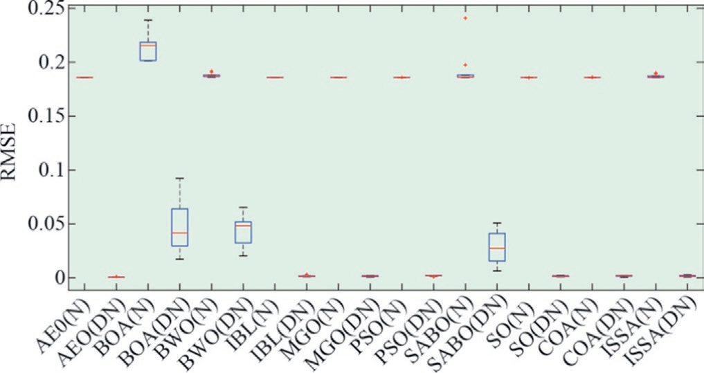
Fig.7.Boxplot of RMSEs obtained by 10 MhAs for SDM under noisy and denoised data.

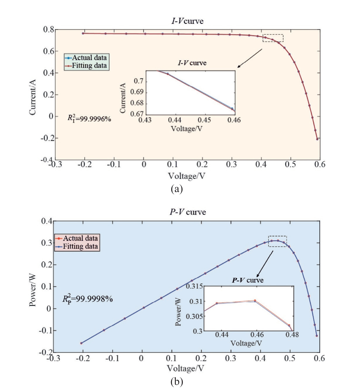
Fig.8.AEO for fitting curves based on denoised data of SDM: (a) I-V curve; (b) P-V curve.

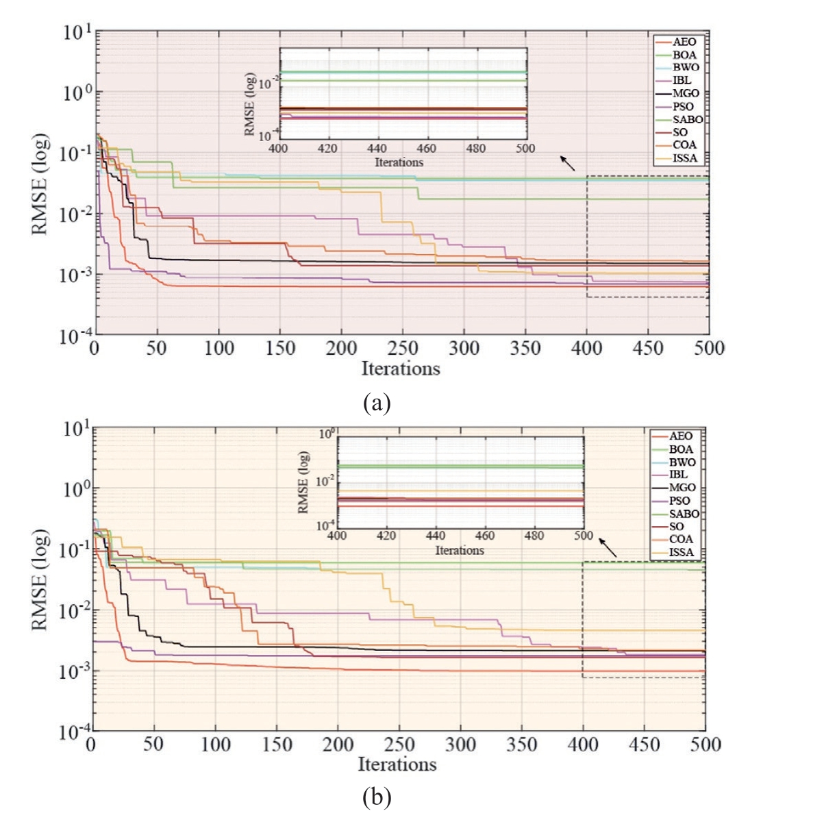
Fig.9.Convergence curves of RMSEs obtained by 10 MhAs for SDM under original and predicted data: (a) Predicted data; (b) original data.

Table 9
Parameter-identification results of original and predicted data based on 10 MhAs for SDM.

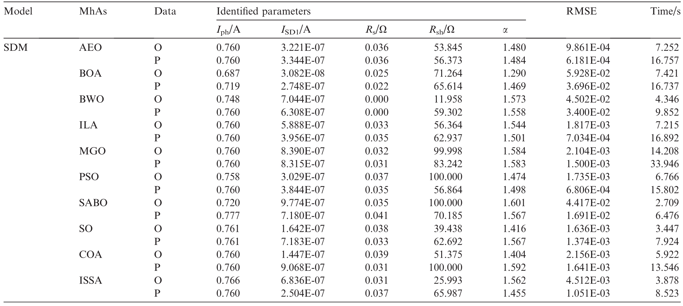
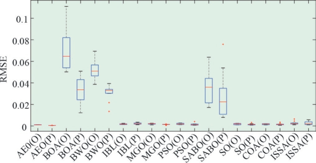
Fig.10.Boxplot of RMSEs obtained by 10 MhAs for SDM under original and predicted data.

2.5 Comparative time-complexity analysis

When analyzing the time complexity of the BNN-AEO,tone must consider the costs of BNN training, algorithm initialization, and the main loop.The training cost of the BNN is high and is expressed as O(E*P*N^2), where E is the number of training epochs, P is the number of parameters, and N is the number of neurons per layer,which depends on the network structure and amount of training data.The initialization phase of the algorithm involves randomly selecting individuals and evaluating the objective function with time complexities of O(n*d)and O(n*C_obj), respectively.Here, n is the population size, d the dimension, and C_obj the cost of the objective function.The main loop is based on the maximum number of function evaluations.Therefore,the total time complexity of the BNN-AEO is approximately O(Max_Sun-Eval*(n*d + n*C_obj) + E*P*N^2).

3 Case studies

This section considers several conventional models such as the SDM, DDM, and TDM on commercial R.T.C.France silicon solar cells, as well as the PV module Photowatt-PWP201 with 36 polycrystalline silicon cells in a series system, were validated using two datasets.The specific data are listed in Table 4.Table 5 lists the prototype parameter values of the two PV models considered in this study.

Subsequently, the BNN and 10 MhAs including AEO,butterfly optimization algorithm(BOA)[34],beluga whale optimization (BWO) [35], intelligible-in-time logics algorithm (ILA) [36], mountain gazelle optimizer (MGO)[37], particle swarm optimization (PSO) [38], subtraction average based optimizer (SABO) [39], snake optimizer(SO) [40], crayfish optimization algorithm (COA) [41],improved salp swarm algorithm (ISSA) were used to extract the parameters of four PV cell models.The main parameters of each MhA are listed in Table 6.Before MhA-based parameter identification was performed, the trained BNN was used to predict, denoise, and add noise to the obtained data.Using the prediction, noisy,denoised, and original data, 10 MhAs were employed to identify the parameters of the four different PV models.Table 7 presents the operating conditions of the PV model.

3.1 SDM parameter extraction

3.1.1 Noise-reduction data

Table 8 summarizes the recognition results of the PV cell parameters obtained using 10 MhAs with different training data.The symbols ‘‘N” and ‘‘DN” represent theresult obtained using noised and denoised data, respectively.As shown in Table 8, after data denoising, the RMSE values of the MhAs were smaller than those under noisy data, among which AEO experienced the most significant decrease of 99.69%.By contrast, the decrease shown by the BOA was the least, (80.07%), followed by BWO (83.00%), the ILA (99.21%), the MGO (98.96%),PSO (98.95%), the SABO (84.39%), the SO (98.93%), the COA (98.76%), and the ISSA (99.13%).

Table 10
Parameter-identification results of noisy and denoised data based on 10 MhAs for DDM.

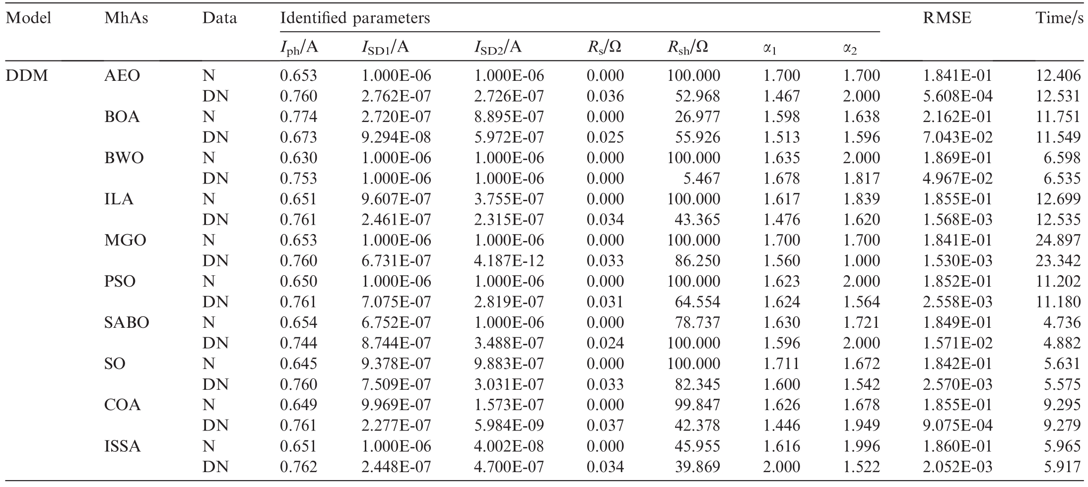
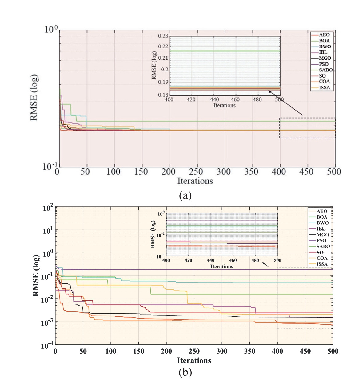
Fig.11.Convergence curves of RMSEs obtained by 10 MhAs for DDM under noisy and denoised data: (a) noisy data; (b) denoised data.

To comprehensively present the convergence performance throughout the iterations of all the algorithms,Fig.6 presents the RMSE convergence curves.The results obtained based on denoised data show higher convergence accuracy, stability, and speed than those obtained using noisy data.

To intuitively compare the optimization accuracy of all methods based on the result distributions between two different training datasets,the RMSE distribution map for 10 iterations was plotted in a boxplot graph, as shown in Fig.7.As shown, after data denoising, all the MhAs showed a smaller distribution range in terms of the lower and upper limits, and the outliers were either reduced or eliminated.This proves that all 10 MhAs exhibited higher optimization accuracy and stability in terms of parameter identification after data denoising.

Fig.8 shows the I-V and P-V characteristic curves obtained by fitting the MhA with the best iterative performance among the 10 MhAs under denoised data.The fitted data curve almost matched the actual data curve almost perfectly.The overlap degree of the I-V curve was 99.9996%, and that of the P-V curve R2P was 99.9998%, thus indicating that the parameteridentification results are consistent with expectations.

3.1.2 Insufficient data

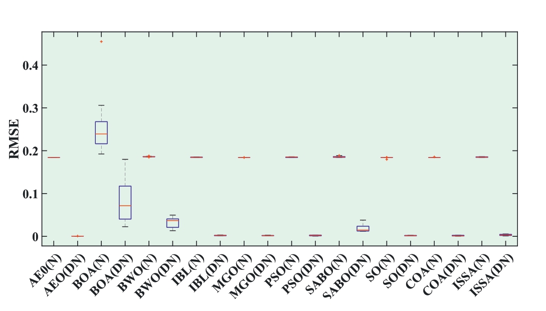
Fig.12.Boxplot of RMSEs obtained by 10 MhAs for DDM under noisy and denoised data.

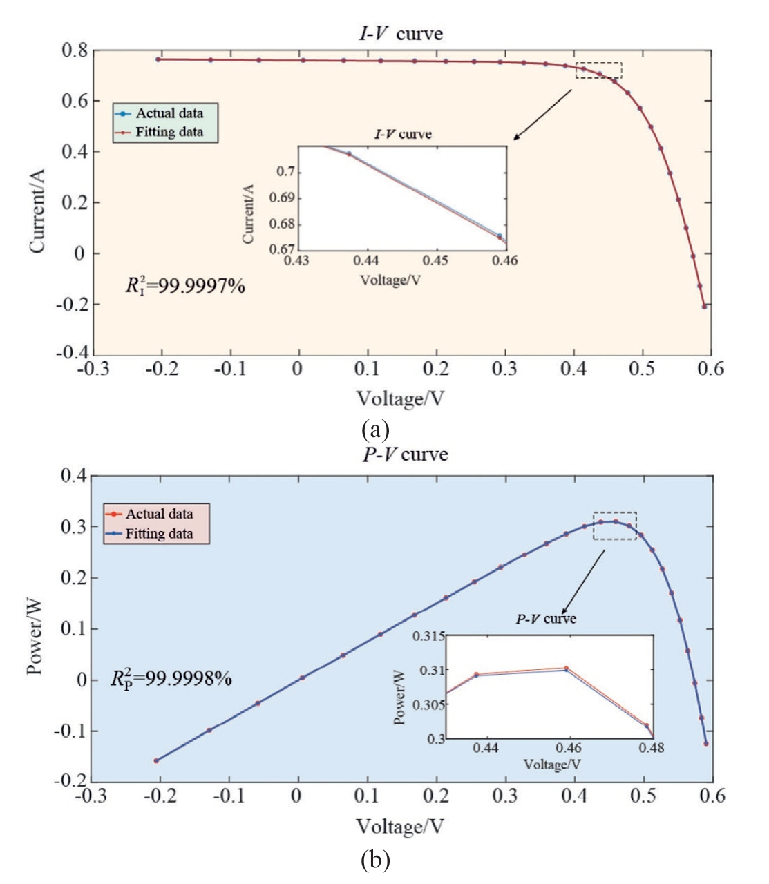
Fig.13.AEO for fitting curves based on denoised data of DDM:(a) I-V curve; (b) P-V curve.

Table 11
Parameter-identification results of original and predicted data based on 10 MhAs for DDM.

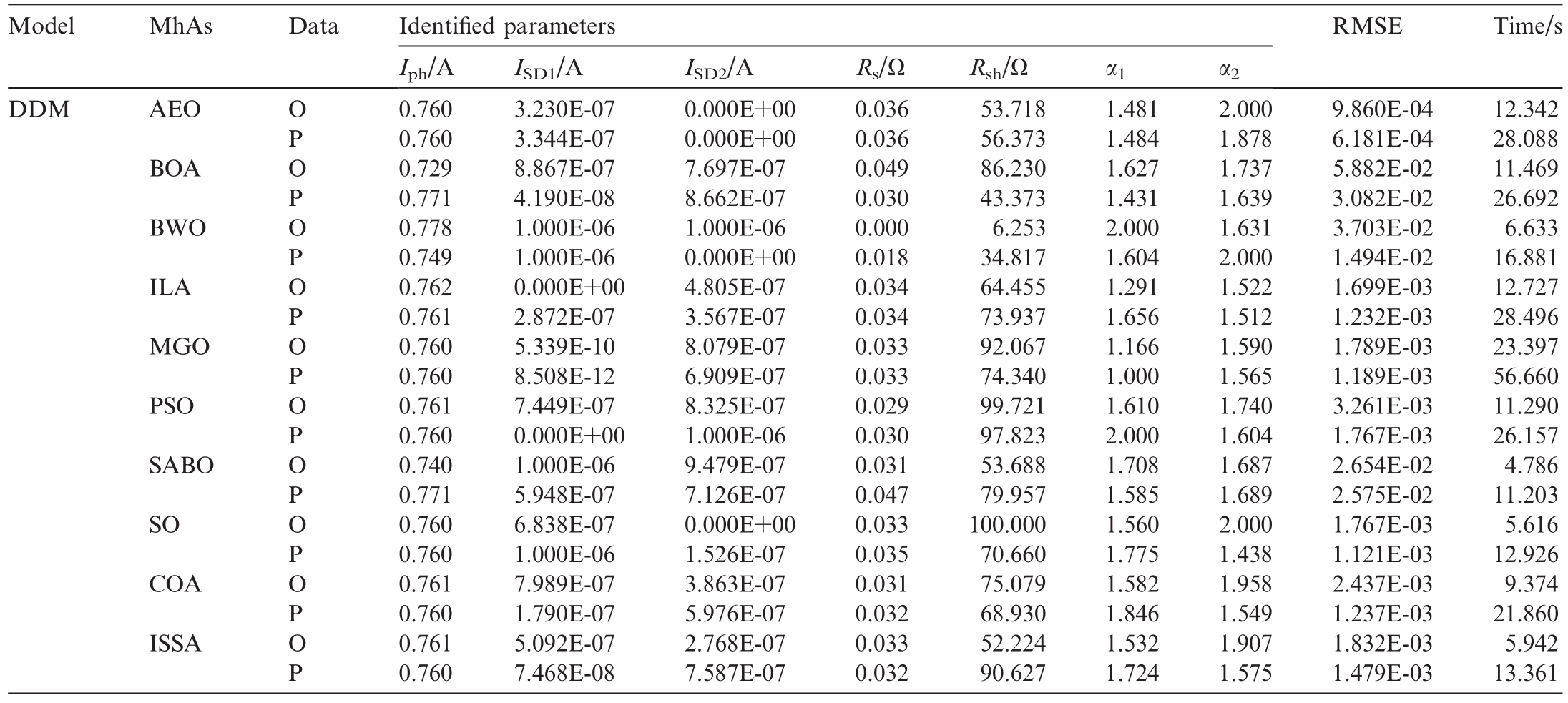
Table 9 summarizes the identification results of the PV cell parameters obtained using 10 MhAs with different training data.The symbols ‘‘O” and ‘‘P” represent the original and predicted data, respectively.Among them,the ISSA indicated the highest decrease of 76.71%,whereas the SO indicated the lowest decrease of 15.96%.Meanwhile, the decreases for the other eight MhAs were as follows: AEO, 37.31%; BOA, 37.65%; BWO, 24.48%;ILA, 61.30%; MGO, 28.71%; PSO, 60.79%; SABO,61.71%; and COA, 23.86%.

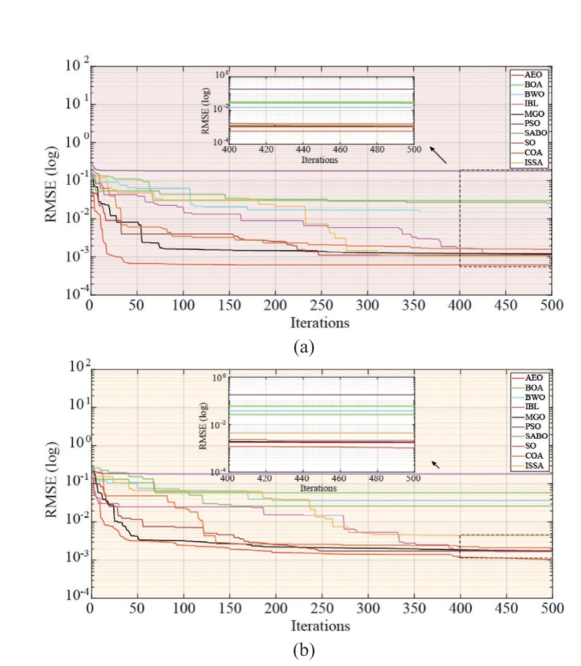
Fig.14.Convergence curves of RMSEs obtained by 10 MhAs for DDM under original and predicted data: (a) predicted data; (b) original data.

Based on Fig.9, the predicted data showed smaller errors than the original data.

As shown in Fig.10,except for the ILA,the upper and lower bounds as well as the median values of RMSE obtained based on the predicted data decreased compared with those under the original data.

3.2 DDM parameter extraction

3.2.1 Noise-reduction data

As shown in Table 10,the decrease shown by AEO was the highest, i.e., 99.70%, whereas that indicated by the BOA was the lowest, i.e., 67.43%.Meanwhile, the decreases indicated by the other eight MhAs were as follows: BWO, 73.43%; ILA, 99.15%; MGO, 99.17%; PSO,98.62%; SABO, 91.50%; SO, 98.60%; COA, 99.51%; and ISSA, y 98.90%.

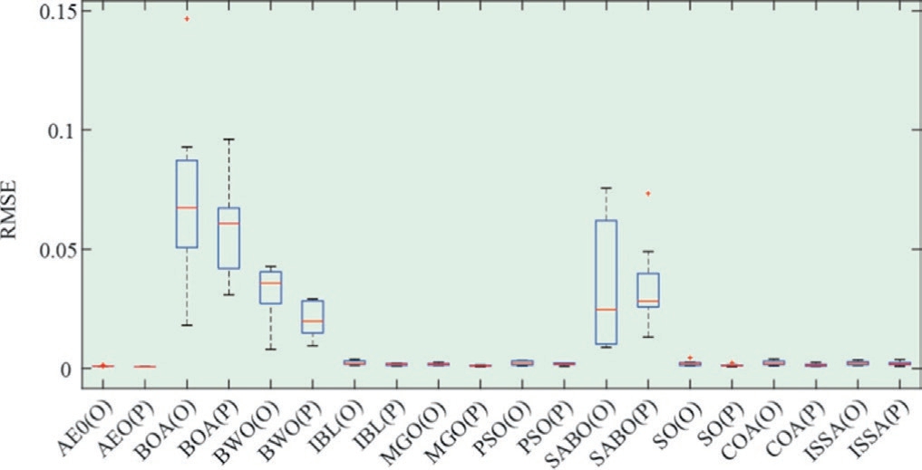
Fig.15.Boxplot of RMSEs obtained by10n MhAs for DDM under original and predicted data.

Table 12
Parameter-identification results of noisy and denoised data based on 10 MhAs for TDM.

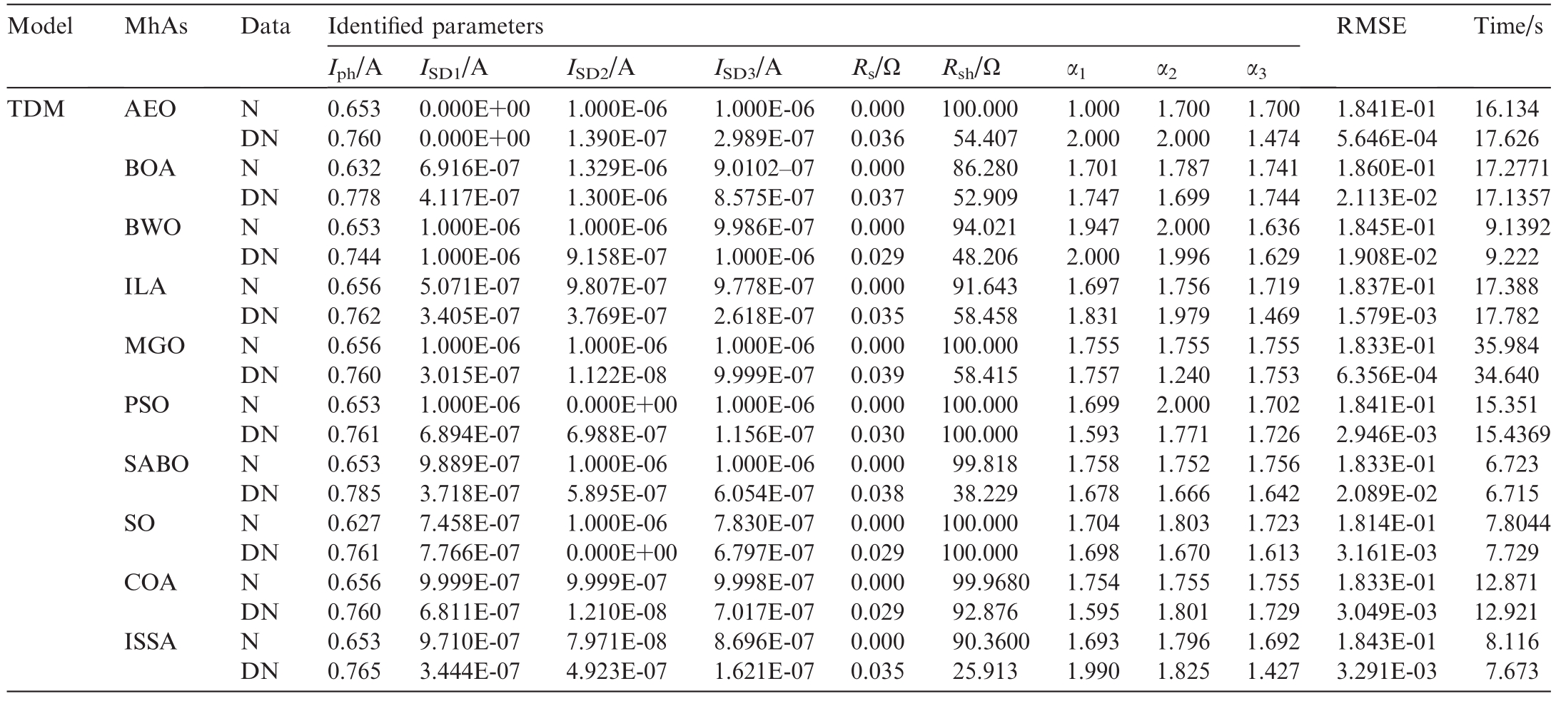
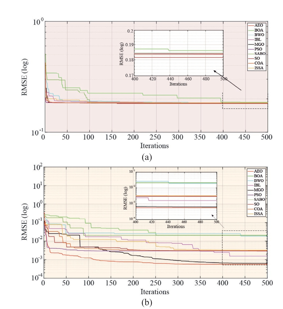
Fig.16.Convergence curves of RMSEs obtained by 10 MhAs for TDM under noisy and denoised data: (a) noisy data; (b) denoised data.

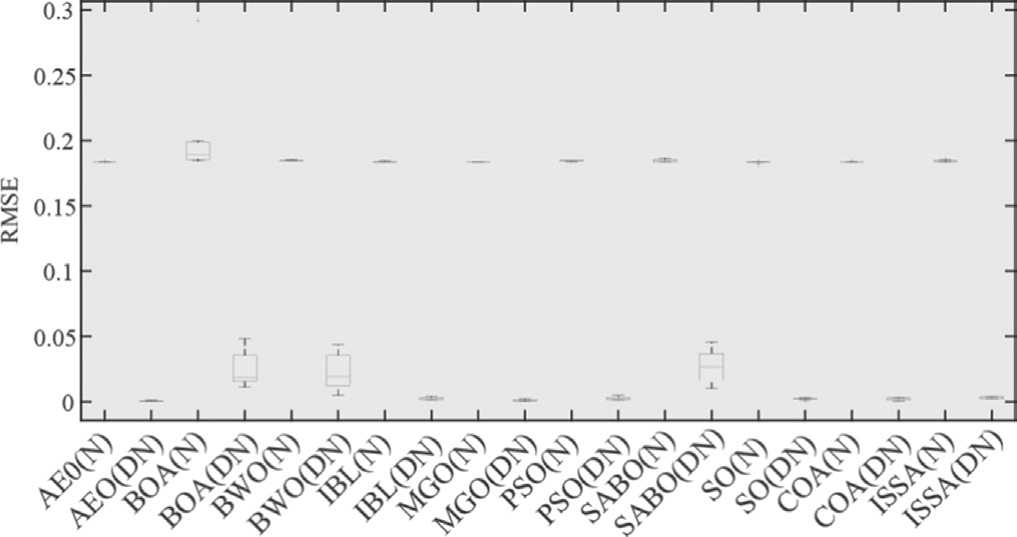
Fig.17.Boxplot of RMSEs obtained by 10 MhAs for TDM under noisy and denoised data.

Fig.11 shows that the RMSE based on the denoised data for 10 MhAs was smaller than that based on noisy data, although the curve convergence based on noisy data was faster.For example, the ILA converged in approximately 50 and 400 iterations under noisy and denoised data, respectively.

To obtain a clear comparison between the two different training datasets, the RMSE values for 10 iterations were plotted in a boxplot graph and the RMSE distribution map was obtained, as shown in Fig.12.The result shows that after data denoising, the upper and lower bounds as well as the median values of the RMSE for each MhA in the boxplot decreased significantly,thus proving that data denoising can improve the stability of MhAs in PV-cell DDM parameter recognition.

Based on Fig.13, the R2 I and R2P were 99.9997% and 99.9998%, respectively, thus indicating that the PV-cell DDM parameter-identification results satisfied the expectations.

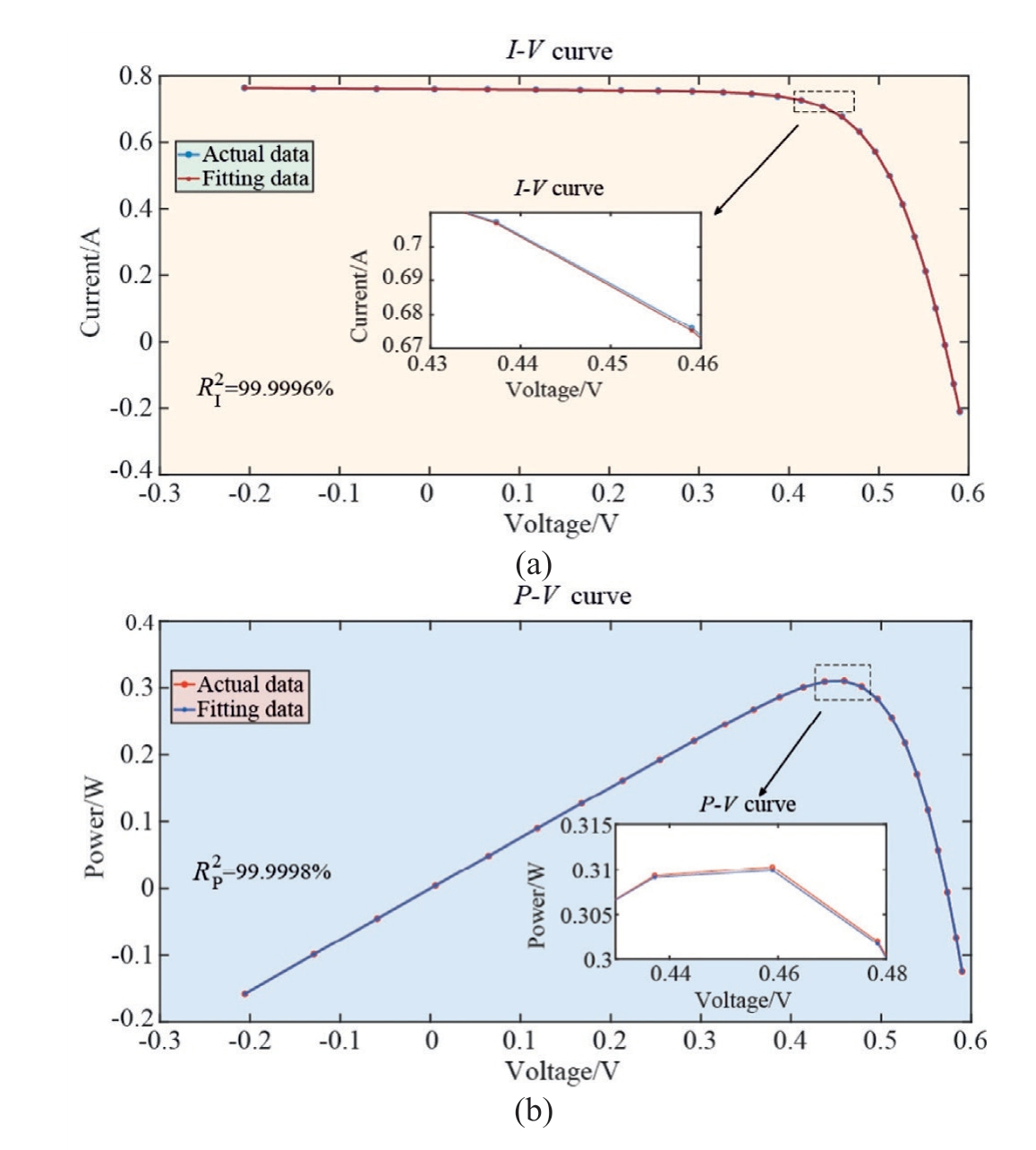
Fig.18.AEO for fitting curves based on denoised data of TDM: (a) I-V curve (b) P-V curve.

3.2.2 Insufficient data

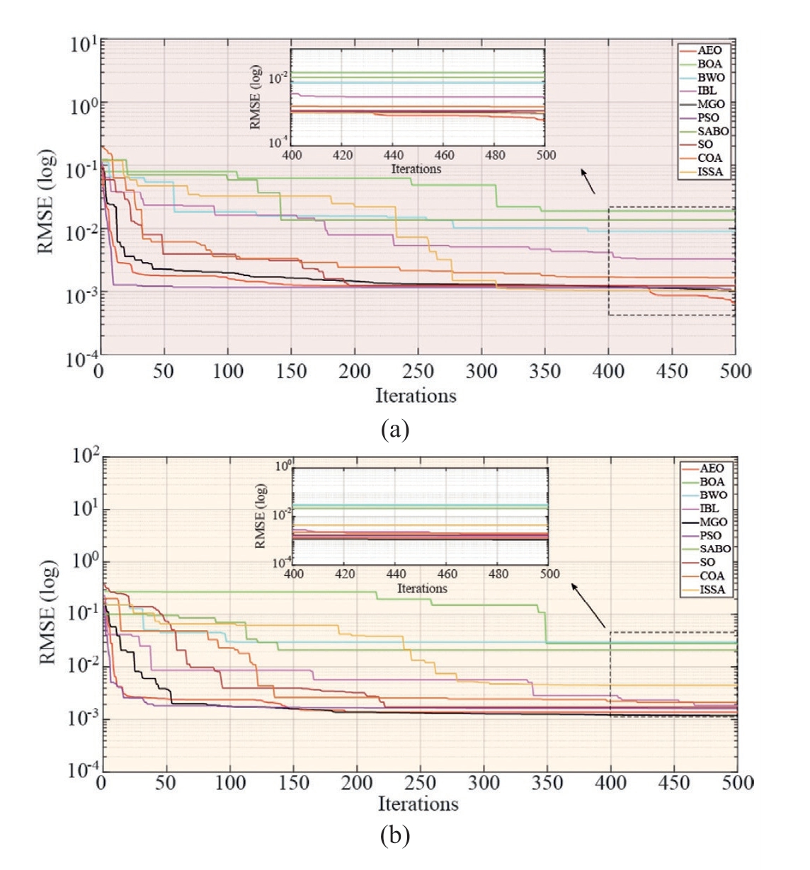
Fig.19.Convergence curves of RMSEs obtained by 10 MhAs for TDM under original data and predicted data: (a) predicted data; (b) original data.

Based on Table 11, BWO and BOA showed significant decreases; for example, BWO indicated the highest decrease of 59.65%, whereas SABO showed the lowest decrease of 2.96%.Meanwhile, the decreases shown by the other eight MhAs were as follows: AEO, 37.31%;BOA,47.60%;ILA,27.44%;MGO,33.52%;PSO,45.80%;SO, 36.57%; COA, 49.26%; and ISSA, 19.26%.

Table 13
Parameter-identification results of original and predicted data based on 10 MhAs for TDM.

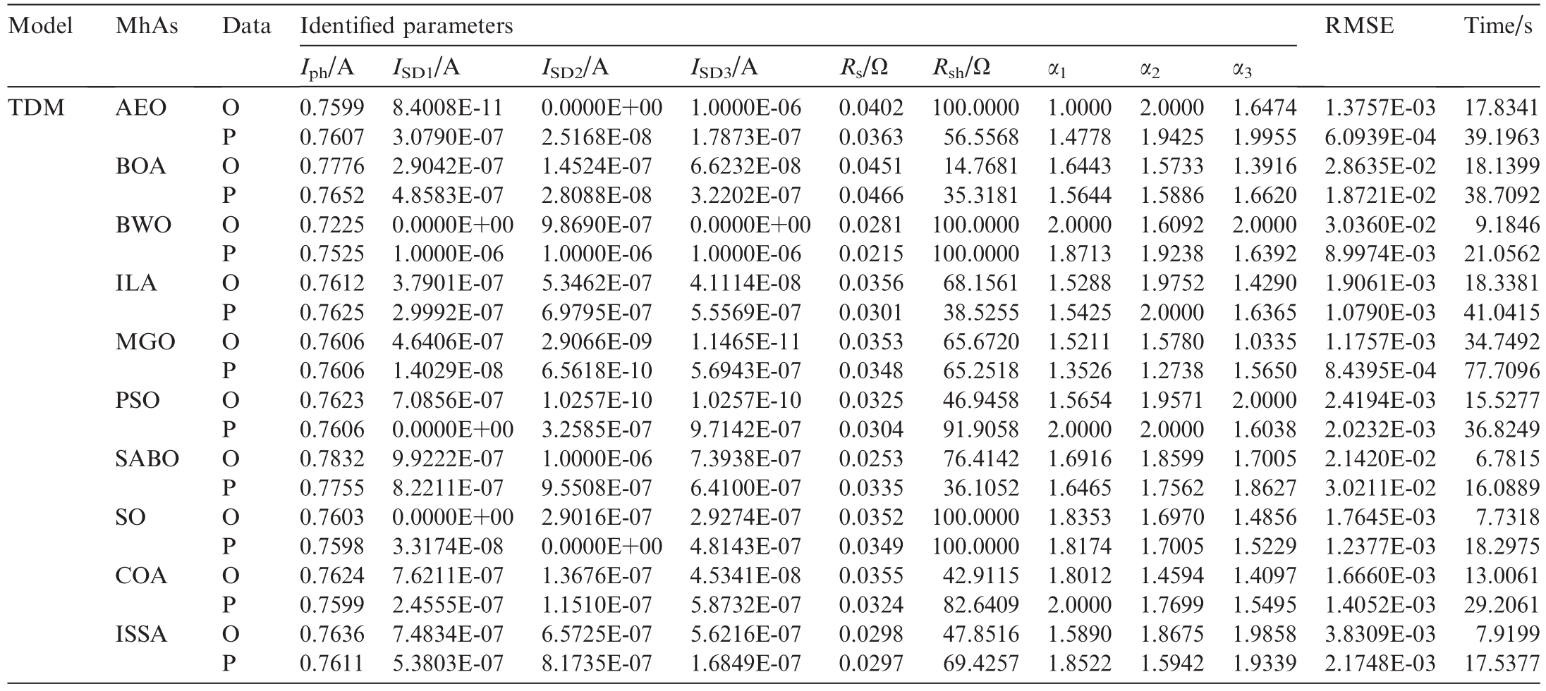
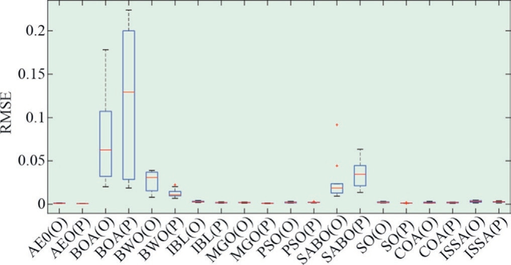
Fig.20.Boxplot of RMSEs obtained by 10 MhAs for TDM under original and predicted data.

Based on Fig.14,after data prediction,the RMSE of all the algorithms decreased.However,the convergence speed of the curve between the two scenarios differed minimally.Based on observation, the data processing improved only the accuracy.

Based on Fig.15, except for the abnormal upper and lower bounds of the RMSE in the BOA,the upper,lower,and median RMSE obtained from the other MhAs based on the predicted data decreased.

3.3 TDM parameter extraction

3.3.1 Noise-reduction data

Table 12 presents the parameter-recognition results of the TDM using 10 MhAs with different training data.Among them, AEO showed the highest decrease of 99.69%, whereas SABO showed the lowest decrease of 88.60%.Meanwhile, the decreases shown by the other eight MhAs were as follows: BOA, 88.64%; BWO,89.65%; ILA, 99.14%; MGO, 99.65%; PSO, 98.40%;SABO, 88.60%; SO, 98.26%; COA, 98.34%; and ISSA,98.21%.

As shown in Fig.16,the RMSE values of the 10 MhAs under denoised data were smaller and accurately reflected the performance differences among the MhAs.The curve values of AEO were the lowest,whereas the curves of each MhA did not differ significantly under noisy data.

The RMSE boxplots of the 10 MhAs shown in Fig.17 indicate that after data denoising, the upper and lower bounds as well as median values of the RMSE for each MhA decreased significantly.All 10 MhAs proved that data denoising can improve the accuracy of MhAs in PV-cell parameter recognition via the TDM.

As shown in Fig.18, the and  were 99.9997% and 99.9998%, respectively, thus indicating that the identification results of the TDM parameters for PV models based on noise-reduction data are consistent with expectations without significant errors.

3.3.2 Insufficient data

Table 13 summarizes the recognition results of 10 MhAs for the TDM parameters of the PV models under different training data.Among them, BWO indicated the highest decrease of 70.36%, whereas PSO indicated the lowest decrease of 16.38%.The decreases indicated by the other eight MhAs were as follows: AEO, 55.70%;BOA, 34.62%; ILA, 43.39%; MGO, 28.22%; SABO,36.43%; SO, 29.86%; COA, 15.66%; and ISSA, 43.23%.

Table 14
Parameter-identification results of noisy and denoised data based on 10 MhAs for PV module.

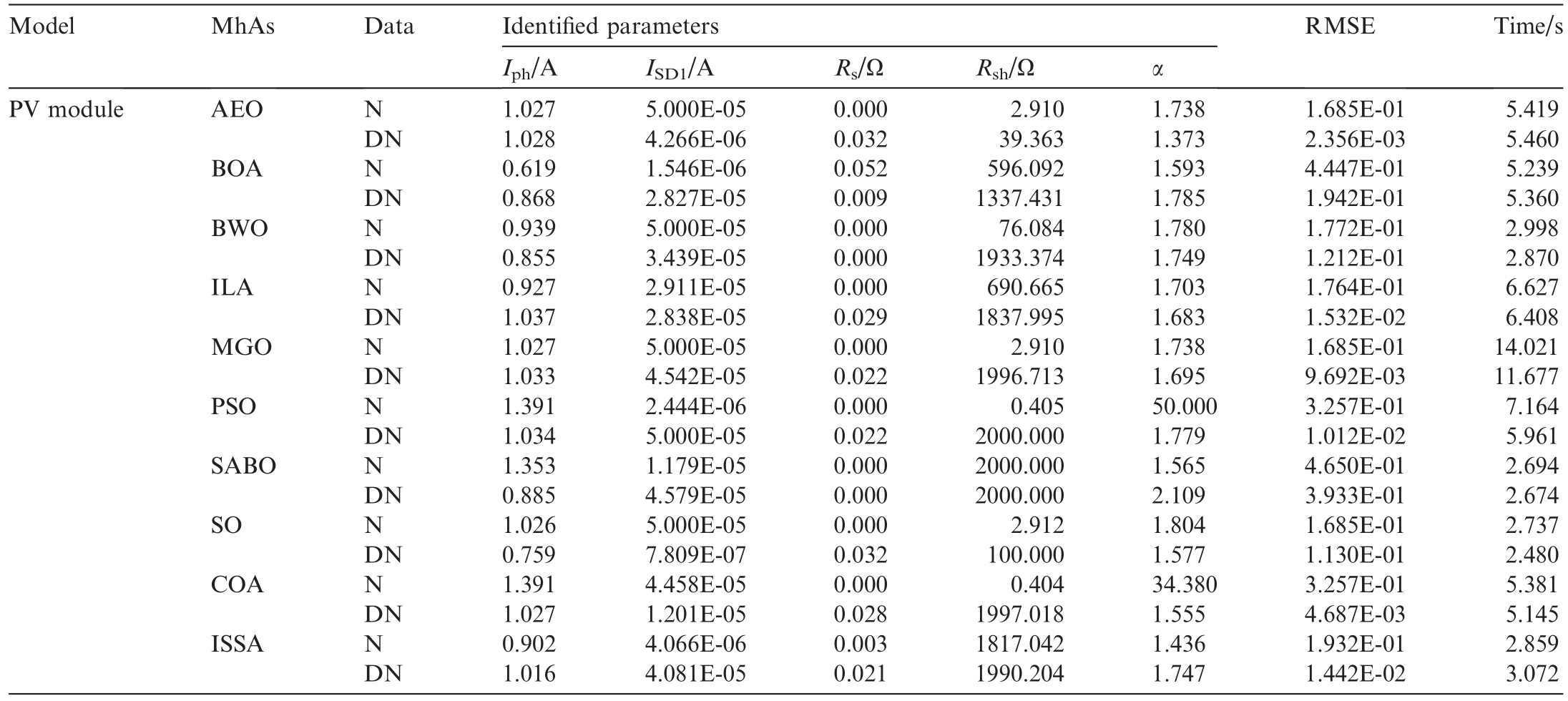
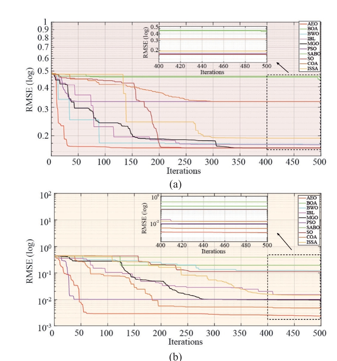
Fig.21.Convergence curves of RMSEs obtained by 10 MhAs for PV module under noisy and denoised data:(a)noisy data;(b)denoised data.

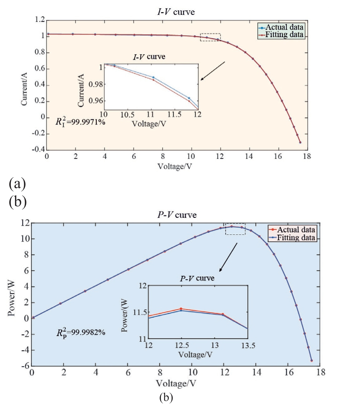
Fig.23.AEO for fitting curves based on denoised data of PV module:(a)I-V curve; (b) P-V curve.

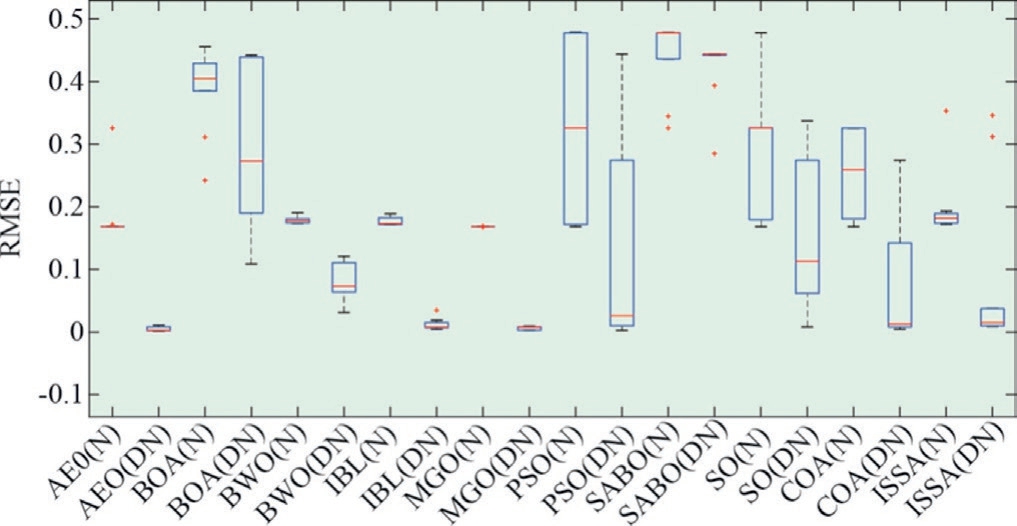
Fig.22.Boxplot of RMSEs obtained by 10 MhAs for PV module under noisy and denoised data.

As shown in Fig.19, after data prediction, the RMSE achieved by all the algorithms decreased.Although the convergence of each MHA in either case differed minimally,the performance difference of each MHA was more pronounced in the predicted data, with no curve overlap.

As shown in Fig.20, except for the upper limit of the RMSE in BOA and the lower limit and median values of SABO, the upper limit, lower limit, and median values of the RMSE obtained from the other MhAs based on the predicted data decreased.

3.4 PV module under variable temperature

3.4.1 Noise-reduction data

Table 14 lists the parameter-recognition results of the PV module using 10 MhAs with different training data.COA indicated the highest decrease of 98.56%, whereas SABO indicated the lowest decrease of 15.43%.Meanwhile, the decreases indicated by the other eight MhAs were as follows: AEO, 98.19%; BOA, 56.33%; BWO,31.57%; ILA, 91.31%; MGO, 94.25%; PSO, 94.12%; SO,32.94%; and ISSA, 92.53%.

As shown in Fig.21,the RMSE values of the 10 MhAs under denoised data were smaller and reflected the performance differences among the MhAs more accurately.Under both noisy and denoised data, the curve values of AEO were significantly lower, and the convergence speed of AEO was higher under denoised data.

The RMSE boxplots of the 10 MhAs presented in Fig.22 show that after data denoising, the upper and lower bounds as well as the median values of the RMSE for each MhA decreased significantly.All 10 MhAs confirmed that data denoising can improve the accuracy of MhAs in PV module parameter recognition.

Table 15
Parameter-identification results of original and predicted data based on 10 MhAs for PV module.

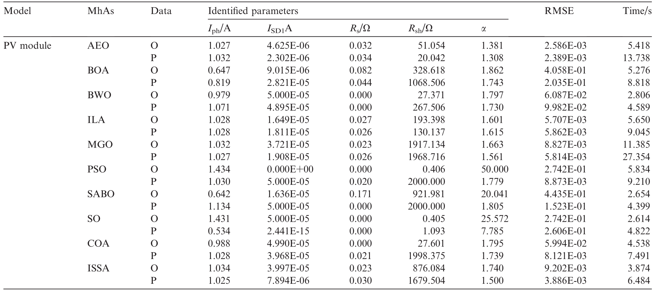
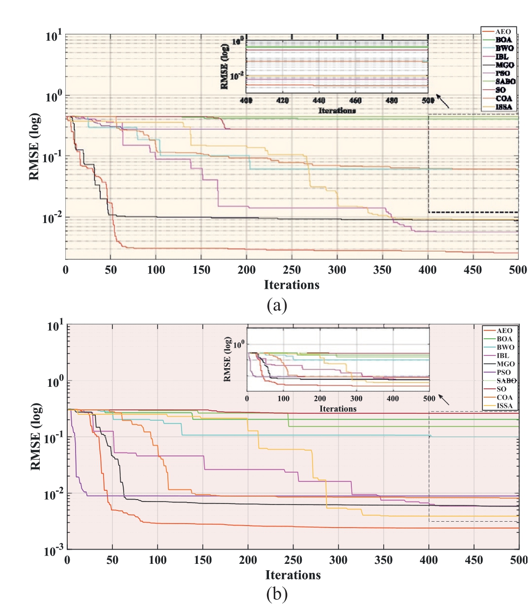
Fig.24.Convergence curves of RMSEs obtained by 10 MhAs for PV module under original and predicted data:(a)predicted data;(b)original data.

Based on Fig.23, the R2I and R2P were 99.9971% and 99.9982%, respectively, thus indicating that the identification results of the PV module parameters on the noisereduction data are consistent with expectations without significant errors.

3.4.2 Insufficient data

Table 15 summarizes the recognition results of 10 MhAs for the TDM parameters of the PV models under different training data.Among them, PSO indicated the highest decrease of 96.76%,whereas SO indicated the lowest decrease of 4.96%.Meanwhile,the decreases shown by the other eight MhAs were as follows: AEO, 20.91%;BOA, 49.84%; MGO, 34.13%; SABO, 65.65%; COA,86.45%; and ISSA, 57.76%.Among them, BWO and ILA showed significant instability, with the RMSE increasing by 63.98% and 2.72%, respectively.

As shown in Fig.24, after data prediction, the RMSE achieved by all the algorithms decreased.Under the two types of data, AEO offered the highest convergence speed and accuracy.

Fig.25 shows that the upper,lower,and median values of the RMSE obtained from the other MhAs based on the predicted data decreased.

3.5 Model sensitivity analysis

A robust metaheuristic algorithm model typically exhibits low sensitivity to parameters.Considering the SDM as an example, parameter sensitivity tests were conducted on the constructed AEO model using the control variable method while ensuring that the remaining parameters and training and testing data remained unchanged.The selected sensitivity testing parameters included C.The population size and maximum number of iterations were retrained and tested by floating them up and down by 20% to compare their changes in testing accuracy.The results are shown in Fig.26.Overall, the sensitivity of the AEO model to the aforementioned parameters was relatively weak, and even when the aforementioned parameters fluctuated by 20%, the RMSE of its testing fluctuated around 0.001.The RMSE of the first two parameters remained relatively constant.The larger the maximum iterations,the smaller was the RMSE,thus indicating that the number of iterations affects the AEO algorithm.

4 Discussion

Radar charts were used to rate each MhA to demonstrate its performance.The radar map was designed to display the five RMSE indicators obtained based on denoised data for 10 types of MhAs, namely, the minimum, maximum, standard deviation, median, and mean RMSEs.

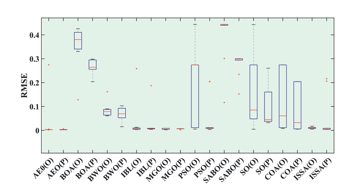
Fig.25.Boxplot of RMSEs obtained by 10 MhAs for PV module under original and predicted data.

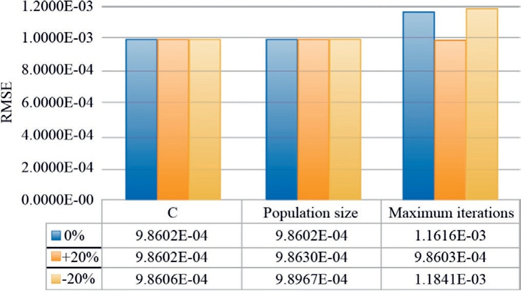
Fig.26.Comparison of testing accuracy of BNN-AEO key parameters with 20% fluctuations in SDM.

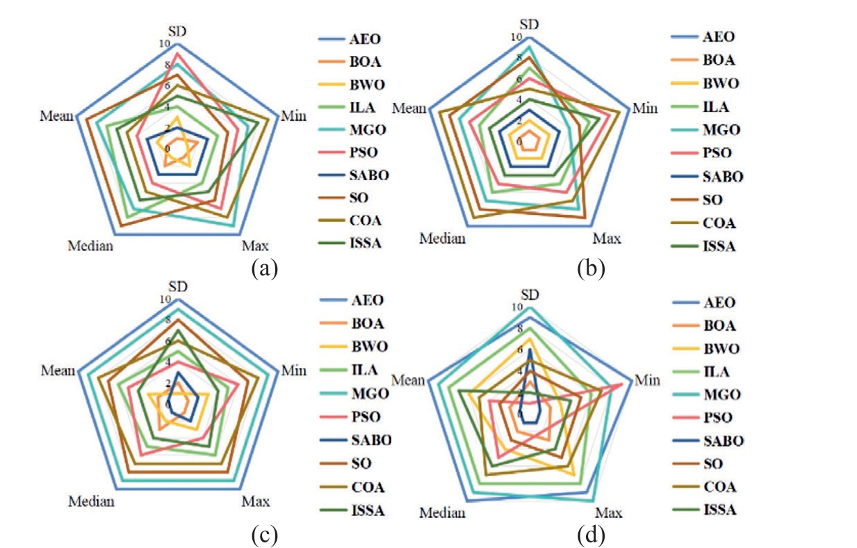
Fig.27.Radar maps of five RMSEs for 10 MhAs of four models under denoised data: (a) SDM; (b) DDM; (c) TDM; (d) PV module.

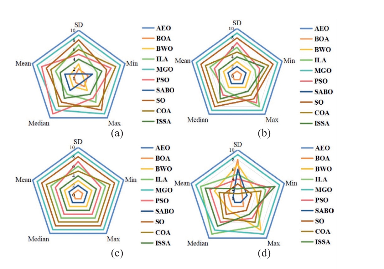
Fig.28.Radar maps of five RMSEs for 10 MhAs of four models under predicted data: (a) SDM; (b) DDM; (c) TDM; (d) PV module.

The higher the score, the lower was the RMSE value of the algorithm and the better was the parameter identification.Based on Fig.27(d), the maximum RMSE and standard deviation scores of AEO were not the highest.However,Fig.27(a),(b),and(c)show that the five RMSE indicators of AEO were lower than those of the other nine MhAs, thus indicating that AEO offers the highest accuracy in identifying the PV model parameters among the 10 MhAs.Similarly, based on the predicted data (see Fig.28), the AEO demonstrated absolute accuracy in PV parameter identification.In summary, after being processed by the BP neural network, the ability of AEO to identify the parameters of the PV models was much greater than that of the other MhAs.

5 Conclusion

A PV-system parameter-identification method for AEO based on a BNN was introduced herein.A BNN was used for data preprocessing to mitigate the adverse effects of data noise, insufficiency, and loss.Subsequently, AEO was performed to identify the parameters of the four PV models.The experimental results indicated that data denoising and prediction improved the accuracy of parameter recognition.Compared with the algorithms proposed in recent literature, AEO demonstrated the highest accuracy and reliability.Additionally, the purpose of extracting PV model parameters was to improve the optimization and control of actual solar energy systems.Under the predicted data, the RMSE values of the SDM, DDM, TDM, and PV modules generated by AEO were 6.1815E-04, 6.1815E-04, 6.0939E-04, and 2.3891E-03, respectively.

Therefore, in future studies, BNN-AEO can be used to process current and voltage data in PV cells, thereby improving the accuracy of parameter identification and establishing more stable PV models.

CRediT authorship contribution statement

Bo Yang:Writing -original draft. Ruyi Zheng: Writing- original draft. Yucun Qian: Conceptualization. Boxiao Liang: Data curation. Jingbo Wang: Writing - review &editing.

Declaration of competing interest

The authors declare that they have no known competing financial interests or personal relationships that could have appeared to influence the work reported in this paper.

Acknowledgments

This study was supported by the National Natural Science Foundation of China (62263014) and the Yunnan Provincial Basic Research Project (202301AT070443,202401AT070344).

References

[1]B.Yang, Y.L.Li, J.L.Li, et al., Comprehensive summarization of solid oxide fuel cell control:a state-of-the-art review,Prot.Control Mod.Power Syst.7 (36) (2022) 1-31.

[2]B.Yang, R.Y.Zheng, Y.M.Han, et al., Recent advances and summarization of fault diagnosis techniques for the photovoltaic system: a critical overview, Prot.Control Mod.Power Syst.9 (3)(2024) 36-59.

[3]Y.J.Chen,B.Yang,Z.X.Guo,et al.,Dynamic reconfiguration for TEG systems under heterogeneous temperature distribution via adaptive coordinated seeker,Prot.Control Mod.Power Syst.7(38)(2022) 1-19.

[4]Y.T.Wang, B.Yang, Optimal PV array reconfiguration under partial shading condition through dynamic leader based collective intelligence, Prot.Control Mod.Power Syst.8 (1)(2023) 1-16.

[5]M.A.Gonza´lez-Cagigal, J.A.Rosendo-Macı´as, A.Go´mez-Expo´sito, Estimation of equivalent model of photovoltaic array using unscented Kalman filters, J.Mod Power Syst.Clean Energy 12 (3) (2024) 819-827.

[6]E.B.Dilger, R.V.de Oliveira, Simulation-based approach to assessing short-term power variations of PV power plants under cloud conditions, J.Mod Power Syst.Clean Energy 12 (6) (2024)1837-1848.

[7]X.H.Chen, J.K.Wu, Photovoltaic power short-term prediction based on long short-term memory neural network optimized by northern goshawk optimization algorithm, Shandong Electric Power 51 (10) (2024) 10-17.

[8]D.W.Yu, S.Li, H.H.Liu, et al., Short-term photovoltaic power prediction based on 3DCNN and CLSTM hybrid model,Shandong Electric Power 51 (7) (2024) 10-18.

[9]B.Yang, J.B.Wang, X.S.Zhang, et al., Comprehensive overview of meta-heuristic algorithm applications on PV cell parameter identification, Energy Conver.Manag.208 (2020) 112595.

[10]J.B.Wang, B.Yang, D.Y.Li, et al., Photovoltaic cell parameter estimation based on improved equilibrium optimizer algorithm,Energ.Conver.Manage.236 (2021) 114051.

[11]H.X.You, Analysis of factors influencing the efficiency of photovoltaic power generation, Energy Technol.Manag.47 (6)(2022) 147-149.

[12]C.Yue, F.H.Isleem, N.D.Qader, et al., Utilization finite element and machine learning methods to investigation the axial compressive behavior of elliptical FRP-confined concrete columns, Structures 70 (2024) 107681.

[13]G.Srikanth,D.Nimma,S.V.R.Lalitha,et al.,Food security based marine life ecosystem for polar region conditioning:remote sensing analysis with machine learning model, Remote Sens.Earth Syst.Sci.(2024) 1-9.

[14]P.S.Agrawal, P.Jangir, L.Abualigah, et al., The quick crisscross sine cosine algorithm for optimal FACTS placement in uncertain wind integrated scenario based power systems, Results Eng.25(2025) 103703.

[15]H.S.Mohamed, T.Qiong, H.F.Isleem, et al., Compressive behavior of elliptical concrete-filled steel tubular short columns using numerical investigation and machine learning techniques,Sci.Rep.14 (2024) 27007.

[16]P.Jangir, S.P.A.Arpita, et al., A cooperative strategy-based differential evolution algorithm for robust PEM fuel cell parameter estimation, Ionics 1 (2024) 39.

[17]P.Jangir, E.A.Ezugwu, Arpita, et al., Precision parameter estimation in proton exchange membrane fuel cells using depth information enhanced differential evolution,Sci.Rep.14(1)(2024)29591.

[18]P.Jangir, E.A.Ezugwu, K.Saleem, et al., A hybrid mutational Northern Goshawk and elite opposition learning artificial rabbits optimizer for PEMFC parameter estimation,Sci.Rep.14(1)(2024)28657.

[19]P.Jangir,E.A.Ezugwu,K.Saleem,et al.,A levy chaotic horizontal vertical crossover based artificial hummingbird algorithm for precise PEMFC parameter estimation, Sci.Rep.14 (1) (2024)29597.

[20]J.Wang, Y.Ji, H.Liu.Gradient-based and multi-innovation gradient-based iterative algorithms for single-diode photovoltaic cell models.In:2021 40th Chinese Control Conference(CCC),26-28 July 2021, Shanghai, China, pp.1166-1171.

[21]L.Hui, D.K.Qiao, H.C.Lin, et al.Parameters identification of photovoltaic cells based on differential evolution algorithm.In:3rd Annual International Conference on Information Technology and Applications (ITA 2016), 29-31 July 2016, Hangzhou, China, pp.1-5.

[22]X.H.Zhu, J.W.Zhong, N.Shi, et al., Parameters identification of photovoltaic cells based on an improved adaptive particle swarm algorithm, J.Heilongjiang Univ.Sci.Technol.32 (6) (2022) 784-789.

[23]B.Liu, Z.K.Tan, S.Q.Tang, et al., Photovoltaic cell parameter extraction using data prediction based on a meta-heuristic algorithm, Power Syst.Protect.Control 49 (23) (2021) 72-79.

[24]H.L.Chen,S.Jiao, M.J.Wang,et al., Parameters identification of photovoltaic cells and modules using diversification-enriched Harris hawks optimization with chaotic drifts, J.Clean.Prod.244 (2020) 118778.

[25]Z.Q.Wu, Z.K.Xie, C.Y.Liu, An improved lion swarm optimization for parameters identification of photovoltaic cell models, Trans.Inst.Meas.Control 42 (6) (2020) 1191-1203.

[26]B.Arandian, E.Mahdiyeh, S.Abd Khalid, et al., An effective optimization algorithm for parameters identification of photovoltaic models, IEEE Access 10 (2022) 34069-34084.

[27]E.Mahdiyeh, A.Ehsan, S.T.Seyed Sadr, et al., A novel hybrid algorithm based on rat swarm optimization and pattern search for parameter extraction of solar photovoltaic models, Energy Sci.Eng.10 (8) (2022) 2689-2713.

[28]E.Akbari, M.Mollajafari, H.M.R.Al-Khafaji, et al., Improved salp swarm optimization algorithm for damping controller design for multimachine power system, IEEE Access 10 (2022) 82910-82922.

[29]X.Chen, K.Ding, J.W.Zhang, et al., A two-stage method for model parameter identification based on the maximum power matching and improved flow direction algorithm, Energy Conver.Manag.278 (2023) 116712.

[30]S.Sharma,P.Shokeen,B.Saini,et al.,Exact analytical solutions of the parameters of different generation real solar cells using Lambert W-function: a review article, Invertis J.Renew.Energy 4(4) (2014) 155-194.

[31]C.L.Fan,F.Gao,S.T.Sun,et al.Bayesian neural networks and its application.In: 4th International Conference on Natural Computation (ICNC 2008), 18-20 October 2008, Jian, China, pp.446-450.

[32]B.Yang, D.Y.Li, C.Y.Zeng, et al., Parameter extraction of PEMFC via Bayesian regularization neural network based metaheuristic algorithms, Energy 228 (2021) 120592.

[33]W.G.Zhao, L.Y.Wang, Z.X.Zhang, Artificial ecosystem-based optimization: a novel nature-inspired meta-heuristic algorithm,Neural Comput.Appl.32 (13) (2019) 1-43.

[34]S.Arora, S.Satvir, Butterfly optimization algorithm: a novel approach for global optimization,Soft.Comput.23(3)(2019)715-734.

[35]C.T.Zhong, G.Ling, Z.Meng, Beluga whale optimization: A novel nature-inspired metaheuristic algorithm, Knowl.-Based Syst.251 (2022) 109215.

[36]M.Masoomeh, N.Hosein, Incomprehensible but Intelligible-intime logics:theory and optimization algorithm,Knowl.-Based Syst.264 (2023) 110305.

[37]A.Benyamin,F.G.Soleimanian,K.Nima,et al.,Mountain gazelle optimizer:a new nature-inspired metaheuristic algorithm for global optimization problems, Adv.Eng.Softw.174 (2022) 103282.

[38]M.Premkumar, S.Ravichandran, T.J.T.Hashim, et al., Fitnessguided particle swarm optimization with adaptive Newton-Raphson for photovoltaic model parameter estimation, Appl.Soft Comput.167 (PA) (2024) 112295.

[39]T.Pavel, D.Mohammad, Subtraction-average-based optimizer: a new swarm-inspired metaheuristic algorithm for solving optimization problems, Heliyon 10 (15) (2024) e35382.

[40]F.A.Hashim, A.G.Hussien, Snake Optimizer: a novel metaheuristic optimization algorithm, Knowledge-Based Syst.242(2022) 108320.

[41]D.S.Abdelminaam, A.S.Alluhaidan, F.H.Ismail, et al.,Parameters extraction of the three-diode photovoltaic model using crayfish optimization algorithm, IEEE Access 12 (2024)109342-109354.

Received 15 May 2024;revised 8 January 2025; accepted 3 February 2025

Peer review under the responsibility of Global Energy Interconnection Group Co.Ltd.

E-mail addresses: yangbo_ac@outlook.com (B.Yang),1209074918@qq.com (R.Zheng), 2418879242@qq.com (Y.Qian),liangboxiao30@163.com (B.Liang), JingboWang96@outlook.com (J.Wang).

https://doi.org/10.1016/j.gloei.2025.02.001

2096-5117/© 2025 Global Energy Interconnection Group Co.Ltd.Publishing services by Elsevier B.V.on behalf of KeAi Communications Co.Ltd.This is an open access article under the CC BY-NC-ND license(http://creativecommons.org/licenses/by-nc-nd/4.0/).

Bo Yang is a professor and Ph.D.supervisor in the School of Electric Power Engineering,Kunming University of Technology, and received his Ph.D.degree from the University of Liverpool,UK,in 2015.He has published more than 180 SCI journal papers and 30 EI journal papers.His research interests include smart grid and the optimization and control of new energy systems based on artificial intelligence.

Ruyi Zheng received her B.E.degree from Kunming University of Science and Technology in 2023 and is currently pursuing a master’s degree in power electronics and power drives in the School of Electric Power Engineering,Kunming University of Science and Technology.Her research interests include identification of battery parameters and diagnosis of battery faults.

Yucun Qian received his B.E.degree from Kunming University of Science and Technology in 2022 and is currently pursuing a master’s degree in electrical engineering in the School of Electric Power Engineering, Kunming University of Science and Technology.His research interests include battery parameter identification, lithium battery state of health estimation.

Boxiao Liang received his B.E.degree from Kunming University of Science and Technology in 2023 and is currently pursuing a master’s degree in power electronics and power drives in the School of Electric Power Engineering,Kunming University of Science and Technology.His research interests include the optimization and control of new energy systems based on artificial intelligence.

Jingbo Wang received his master’s degree from Kunming University of Science and Technology in 2022, and was awarded a full scholarship by China Scholarship Council(CSC)to study for a doctoral degree at the University of Liverpool,UK, in 2022.His research interests include modeling and optimization of new energy generation systems.

(Editor Yajun Zou)