0 Introduction

In recent decades,global climate change has impacted traditional energy sources,and mankind has begun to search for and utilize renewable energy sources,such as solar,wind,and hydroelectric power.Compared to traditional energy sources,clean PV energy produces less pollution and is more environmentally friendly.Accurate PV power prediction plays a vital role in the safe and stable operation of power systems.However,PV power generation is susceptible to seasonal changes,weather conditions,and diurnal variations.Furthermore,it has a high degree of randomness and volatility,posing challenges to the stable operation of large-scale power grids.Therefore,an accurate prediction of PV power generation can help the power dispatch department to optimize power grid operations,improve power grid stability,and reduce operating costs.

Currently,PV forecasting is primarily categorized into three temporal scales: short-term (1-3 days),medium-term(3-10 days),and long-term (beyond 10 days).Spatially,forecasts can be made for individual photovoltaic power stations or regional photovoltaic systems as a whole.There are two types of forecasting methods: point and interval.Point forecasts provide a definitive power value for a specific moment;interval forecasts offer a range of uncertainties for the forecasted value,and probabilistic forecasts provide the probability distribution of the forecasted values.PV power prediction models are mainly classified into physical,statistical,and machine learning models.Physical models,such as the NWP [1]model,mainly use geographic and meteorological data to calculate PV power.However,the physical modeling process involves setting several parameters with varying degrees of complexity,and thus,the process may appear cumbersome.Statistical analysis models [2-3] usually describe the relationship between historical time series and forecasted PV power based on a large amount of historical data.Models such as autoregressive integrated moving average (ARIMA) has the advantages of simple construction and high-speed calculation.However,the error is large when dealing with volatile PV data.At present,most research efforts are focused on ultra-short-and shortterm point forecasting for individual photovoltaic power stations.However,there is comparatively less research on medium-to long-term forecasting.Moreover,interval and probabilistic forecasting,which are significant forms of photovoltaic power generation forecasting,continue to be key areas of research for future development.Machine learning models have been successfully applied to PV power prediction because of their powerful nonlinear regression ability to improve the prediction accuracy.Banik et al.[4] combined the random forest and CatBoost algorithms for PV power prediction and improved the accuracy by 6% compared to the baseline model.Ramos et al.[5] designed three prediction methods based on random forest,support vector machine,and gradient boosting to predict the distributed PV grid power in Queensland,Australia.The experimental results showed that the gradient boosting-based model had better robustness and a lower prediction error than the baseline model.Alrashidi et al.[6] used a metaheuristic optimization algorithm to improve the support vector regression and artificial neural networks.Experimental results showed that the root mean square error of the optimized model was reduced by 12.001-50.079%compared with that of support vector regression.Ma et al.[7]proposed a short-term PV power prediction method based on MFA-Elman to solve the problems of stochasticity and slow training speed associated with the initial weights and thresholds of the Elman neural network.Results showed that the MFA-Elman model had the smallest prediction error compared to the baseline model.

However,traditional machine learning models are not capable of capturing the time dependency of PV data,but recurrent neural networks (RNN) are widely used for PV power prediction because of their recurrent structure and parameter-sharing mechanism,which can better capture the time dependency in time-series data.Sharma et al.[8] optimized a long short-term memory (LSTM) model using Nadam.The results showed that the optimized model improved the prediction accuracy by 47.48% compared with that of the seasonal autoregressive integrated moving average (SARIMA) method.Sarkar et al.[9] proposed a hybrid approach based on the random forest (RF) and LSTM.The results of publicly available data showed that the hybrid model combined the advantages of different models,thereby providing higher accuracy.Li et al.[10]proposed a hybrid model combining the Pearson correlation coefficient (PCC),ensemble empirical mode decomposition(EEMD),and sample entropy (SE) (owing to the strong stochasticity and volatility of PV power),with the sparrow search algorithm (SSA) and LSTM hybrid model.Results showed that the PCC-EEMD-SSA-LSTM model has the smallest prediction error compared with the baseline model under different weather conditions.Kothona et al.[11]proposed a combined ELSTM-FFNN model and compared the proposed model with a single LSTM.The results showed that the prediction accuracy improved by 3-11.9% and 0.2-17.8% in two prediction ranges,respectively,proving that the combined model can combine the advantages of a single model to achieve better prediction results.Chen et al.[12]considered the correlation between PV feature variables and first used Pearson coefficients to remove irrelevant features and then used LSTM to model regression prediction on the remaining features.The results showed that the amended model improved the prediction accuracy.Li et al.[13]proposed an LSTM-FC model consisting of LSTM and fully connected (FC) models,which considered not only the effect of meteorological data on power generation,but also the time continuity and cycle dependency.The experimental results showed that the LSTM-FC model improved the RMSE metrics by approximately 11.79% when compared with the support vector machine.

However,LSTM is prone to gradient vanishing or explosion,leading to the degradation of prediction accuracy.However,the transformer can better learn the relationship between PV features through an attention mechanism with good stability and applicability.Tian et al.[14] used a transformer to predict ultra-short-term PV power generation,and experimental results on the Hebei Province PV dataset showed that it improved the mean absolute percentage error(MAPE) by approximately 22.0% and 29.1% compared to gated recurrent unit (GRU) and deep neural networks,respectively,indicating that the GRU has a better prediction capability and stability.Gao et al.[15] used a transformer to consider the correlation between features,such as time and space,temperature,and humidity.The experimental results show that the transformer can improve the average absolute percentage error by approximately 20.9% compared with RNN-like models.Considering that aerosol optical depth(AOD) is the main factor affecting global horizontal irradiance (GHI),Xiu et al.[16] used an informer to predict the GHI for the next 8 h using the AOD,meteorological parameters,and historical GHI data of Beijing as input variables and verified the applicability of the model using Golden data.The experimental results showed that the model can improve the computational efficiency and prediction performance.Cao et al.[17] proposed a combined LSTM-informer model.This model improves the k-fold cross-validation in the traditional stack algorithm to time-series cross-validation and provides accurate shortand medium-term PV power forecasts by integrating the advantages of the two underlying models.Jiang et al.[18]added an additional MLP layer to an autoformer for more efficient deep information extraction.The results on the Pecan Street dataset showed that the model can improve ultra-short-term load forecasting accuracy.

A traditional transformer embeds multiple variables from each time step in the PV data into the same marker,leading to meaningless learned attention maps that do not adequately handle multivariate feature correlations [19].The classical attention mechanism requires quadratic time complexity and high memory usage in the modeling process when faced with long input and output sequences.Therefore,a two-stage PV power prediction model called TSformer is proposed to optimize the transformer.The main contributions of this study are as follows:

1.The first stage of the TSformer model is constructed using an inverted transformer backbone,which learns the complex nonlinear representation of the PV power data through a new inverted perspective and captures the multivariate correlation and volatility between the PV power characteristic variables,thus improving the model prediction performance and generalization ability.

2.Introducing ProbSparse attention to solve the problem of memory and computation occupied by the attention part of the traditional attention mechanism.This increases the square ratio with an increase in sequence length,reduces memory occupation and time overhead during the attention computation process,and improves the computational efficiency of the model.

3.The second stage of the TSformer model consists of a weighted series decomposition module that uses a sequence decomposition unit to extract the photovoltaic power data cycle characteristics.By implementing a weighting mechanism constraint on the series decomposition unit,the model ensures that predictions align more closely with actual patterns of change to improve the accuracy of the model prediction.

4.Experiments were conducted using two publicly available PV power datasets.The results showed that the prediction accuracy of TSformer was better than that of the current popular baseline model,with better prediction performance and computational efficiency.

1 Model structure

TSformer,a two-stage PV power prediction model consisting of first and second stages,is proposed in this paper.The first stage uses an inverted transformer backbone.It optimizes the traditional attention mechanism using ProbSparse attention.The second stage introduces a weighted series decomposition module that considers the physical characteristics of the PV data.In the first stage,raw photovoltaic sequence data are processed to learn the complex nonlinear expressions of the original sequence and capture multivariate correlations and volatilities between variables.It is then mapped to the prediction results and input into the second stage,where temporal features and periodic information are extracted,and the prediction output is generated.

A PV power prediction model was constructed by combining the first and second stages.The architecture of the model is shown in Fig.1.

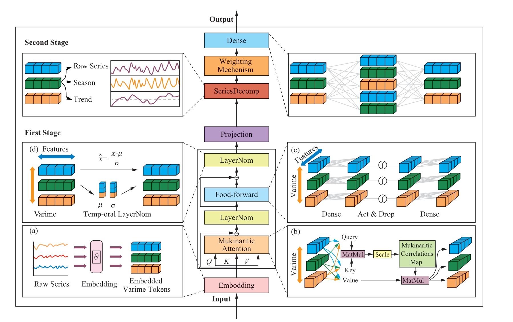
Fig.1 Architecture of the TSformer model

1.1 First Stage

The first stage optimizes the transformer with a new inverted perspective and ProbSparse attention,which inverts the duties of the attention mechanism and feedforward neural network to better handle the multivariate correlations,complex nonlinearities,and volatility of PV data.The inverted transformer backbone first embeds the entire PV sequence independently into variable tokens through an embedding layer,where the embedded tokens aggregate a global representation of the sequence,mapping the entire sequence of the same variable into a high-dimensional feature representation.Second,ProbSparse attention is introduced to reduce the time and memory consumption during the computation of the traditional attention mechanism and thereby improve the computational efficiency.ProbSparse attention was applied to the embedded variable tokens to reveal the multivariate correlations between the variables,followed by extracting the sequence representation of each token using a feedforward neural network,and finally outputting the results of the first stage using a projection layer.

1.1.1 Embedding

Embedding was realized using a multilayer perceptron(MLP).However,unlike a traditional transformer,which uses an embedding operation,positional embedding is no longer required because the feedforward network implicitly stores the positional order of the PV sequence.As shown in Fig.2,first,the entire PV power sequence is embedded independently into variate tokens,where the embedded tokens aggregate the global representation of the sequence;the entire sequence of the same variable is mapped into a high-dimensional feature representation (variate token);second,ProbSparse Attention is applied to the embedded variate token to reveal the multivariate correlation among the variables;then,the sequence representation of each token is extracted using an FFN.

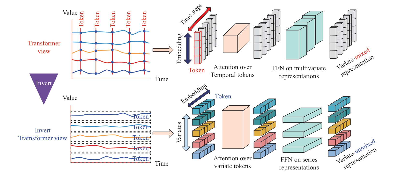
Fig.2 Transformer vs.Invert Transformer

1.1.2 Layer normalization

In a traditional transformer,this module simultaneously normalizes multiple variables in the PV data,resulting in a mishmash of variables that are indistinguishable.Acting layer normalization on the time dimension after inverting the architecture not only reduces the characteristic distribution differences between variables but also solves problems such as the non-stationarity of the PV data,as follows:

where H={h1,… hN }∈RN × Ddenotes N embedded tokens of dimension D;hn denotes the nth token;and Mean(hn) and Var(hn) denote the mean and variance of the input tokens,respectively.

1.1.3 Feed-forward network

In contrast to the original transformer,the inverted version of the transformer embeds each time series as a variable token,applies a feedforward neural network to the sequence representation of each variable token,and encodes sequences to capture multivariate correlations as follows:

where x is the input PV feature vector,W1 and W2 are the trainable weight matrices,b1 and b2 are the trainable bias vectors,and max(0,) denotes the ReLU activation function.

1.1.4 Attention

When modeling multivariate time-series data,the traditional transformer treats each time step as a token,which may not effectively capture the correlation between multiple variables.Instead,the inverted transformer backbone treats the entire sequence of variables as a separate process.It treats each variable feature as a token and applies the attention mechanism between the variables.This inversion is effective in learning the dependencies between multiple time-series variables.In the inverted transformer backbone,the attention module obtains the query,key,and value through linear projection,thus revealing the correlation between multiple variables.In the next representation of the interaction,highly correlated variables are given more weight,which helps the model better capture the correlation information between the variables.The traditional attention mechanism calculates the input attention matrix based on the query,key,and value using a scaled dot product as per the following formula:

where Q ∈represents the query vector,K ∈represents the key vector,V ∈represents the value vector,represents the normalization factor,and Softmax represents the normalization equation.

However,the traditional attention mechanism suffers from sparsity;that is,fewer dot products contribute to the vast majority of the attention score,meaning that the remaining paired dot products can be ignored.To improve the efficiency of the traditional attention mechanism,the sparsity of the query was measured using a KL scattering measure,where the sparsity of the ith query is given by the following formula:

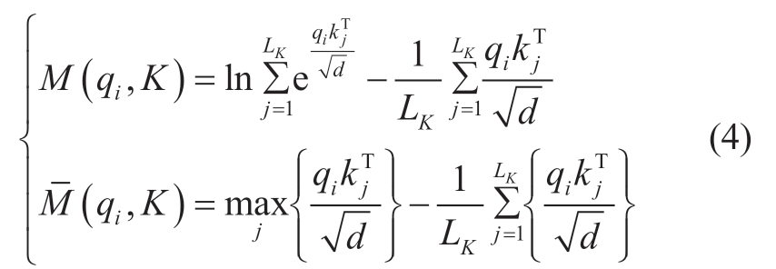
Here,qi is the ith row in the Q matrix,M(qi,K)denotes the sparsity measure of the ith query, (q i,K)denotes the approximate sparsity measure of the ith query,and LK denotes the length of the query vector.

The first u  was set as.Therefore,the formula for the probabilistic sparse attention mechanism is as follows:

Finally,by computing only the Ln(L) moments of ,the complexity can be reduced from O(n2) to O(L·Ln(L)).

1.1.5 Projection

The PV data first uses embedding to obtain variable coding,followed by ProbSparse attention for information interaction between variables.LayerNorm is then applied to unify the feature distribution of different variables,and an FFN is used to obtain an efficient time-series representation,which is finally mapped to the prediction results in the first stage by projection.

1.2 Second Stage

In the second stage,a weighted series decomposition module is proposed in combination with the physical and periodic characteristics of the PV data,which mainly includes the following two parts: (1) Because of the obvious periodicity of the PV power data,a sequence series module is introduced to extract the temporal patterns and periodicity.(2) Considering that the real PV output power is closely related to the sine function change pattern,a weighting mechanism for constraining the output results of the model is proposed to align it with the real PV power changes.

1.2.1 Series decomp

In the field of PV forecasting,numerous studies have aimed to improve the prediction accuracy and reduce the computational costs.Among them,an influential study proposed a fast Fourier transform (FFT) method that performed well [20-21].However,considering the computational costs,we decided to use the moving average method.

When analyzing PV time-series data,the moving average method eliminates random noise by smoothing the PV data,making it easier to identify the trends and seasonal components in the series [22].However,the attention mechanism focuses more on the key parts of the series and does not consider its overall time-series nature.Numerical data lack semantics,and the attention mechanism inevitably loses part of the series information when the modeling trend changes between consecutive points.Therefore,periodic fluctuations can be smoothed by adjusting the moving average to highlight long-term trends.The primary procedure involves selecting a window size and calculating the average of all points within that window for each point in the time series.This average value replaces the original data points,resulting in a new smoothed sequence.After moving the average processing,the transient fluctuations in the sequence are dampened,leaving behind a representation that predominantly captures the long-term trajectory of the data.Consequently,the smoothed sequence embodies the trend component of the original series.Therefore,seasonal and random fluctuations can be represented by subtracting the trend component from the original series.The formula used is as follows:

where xt,and xs denote the trend and seasonal terms,respectively,AvgPool(·) is used to perform moving averages,and Padding(x) denotes a padding operation to keep the sequence length constant.

1.2.2 Weighting mechanism

Incorporating physical constraints when performing PV power prediction tasks can address the drawbacks of machine-learning algorithms that rely solely on large datasets [23].As shown in Fig.3,the Sanyo and Solibro PV power data have the following two distinct characteristics:(1) there is a fixed output of zero for the real PV power and(2) the real PV power has a distinct daily periodicity.Since the real PV power change situation is closely related to the Sin function change pattern,the weighting mechanism was designed on the basis of the Sin function.By comparing the PV power data with the Sin function change situation,the change in the blue shaded area in the Sin function change image in Fig.3 was used as the weight matrix of the prediction result (W).The formula used is as follows:

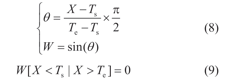
Fig.3 Data distribution characteristics

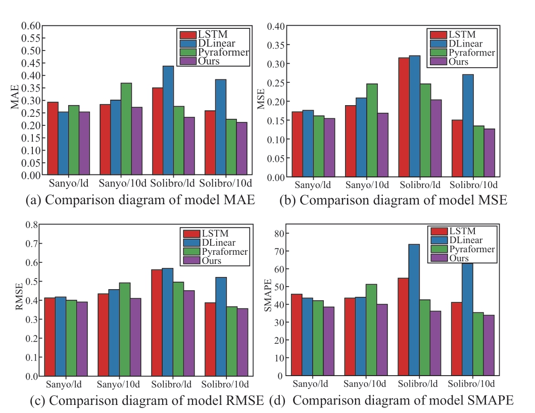
Fig.4 Model performance comparison

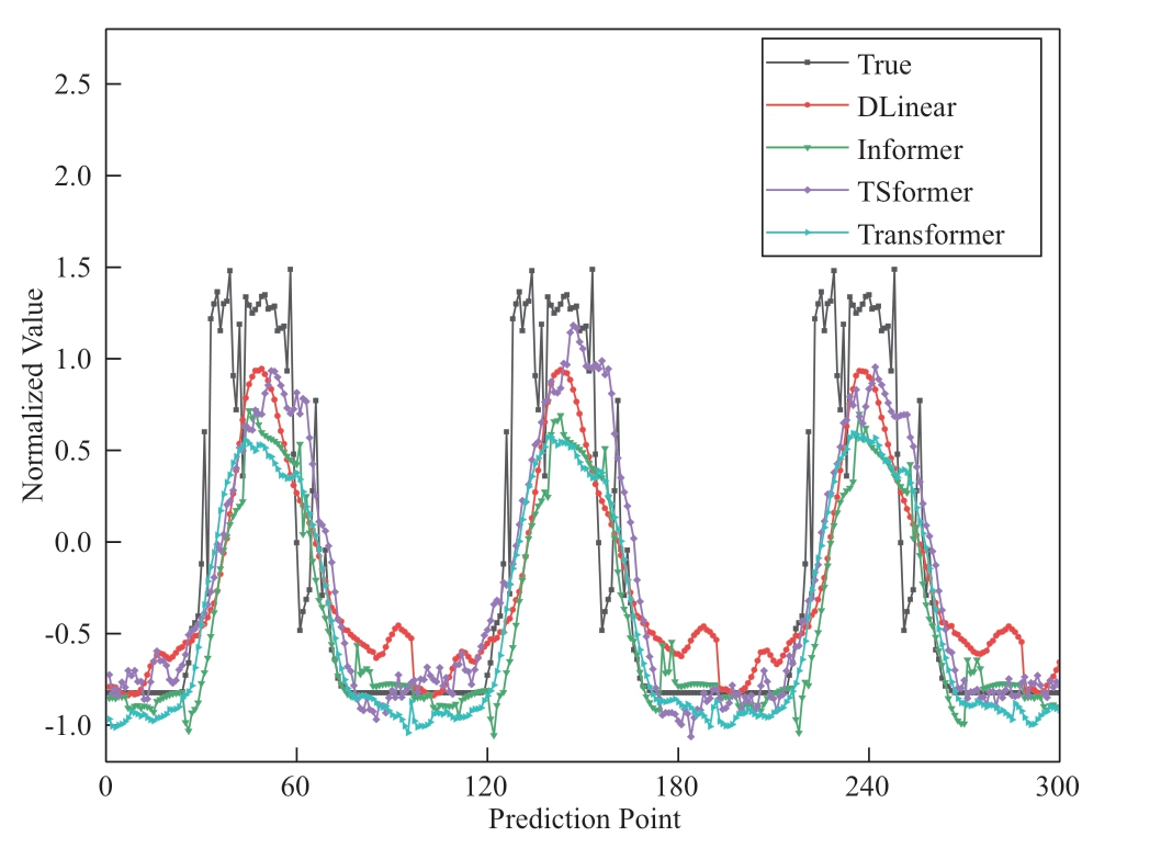
Fig.5 Forecasting results of day one

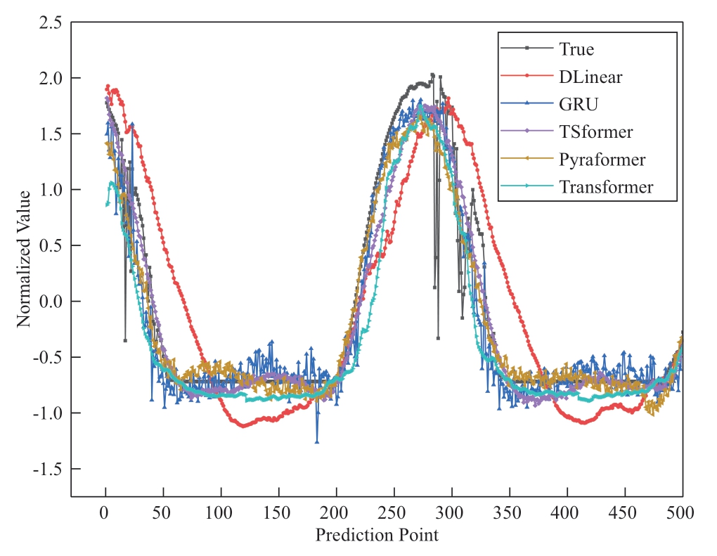
Fig.6 Forecasting results of day 10

Here,Ts and Te are trainable parameters in the model,denoting the start hour and end hour of the time range,respectively;X denotes the current input time data;θ denotes the angle;and W denotes the weight matrix.

The input values are mapped to the interval from 0 to π/2 by using Equation 8,and the weight values are assigned using the sine function.The values that are not within the set range are set to 0 using Equation 9,and finally,the weight W is multiplied with the decomposition tensor of the PV data sequence as the prediction result to improve the model prediction accuracy.Based on the results of the timeseries decomposition,seasonal and trend terms of the PV data were obtained.The seasonal term represents cyclical fluctuations in the PV data caused by seasonal changes,whereas the trend term reflects the long-term trend of the data.The seasonal and trending characteristics obtained from the decomposition provide an important basis and reference for future PV power prediction and analysis.

2 Case Study

2.1 Data Description

In this study,two publicly available PV power datasets from the Alice Springs region of the DKASC PV system in Australia,namely the Sanyo and Solibro power plant datasets,were used to validate the performance of the proposed TSformer model.The time resolution was 15 min,and the forecast steps were 1 and 10 days.These correspond to predictions of 96 and 960 future time steps,respectively.The details of the experimental datasets are listed in Table 1.

Table 1 Description of experimental dataset

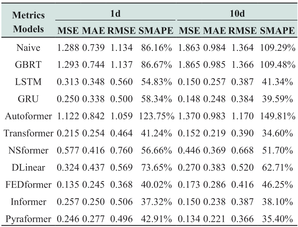
Table 2 Comparison of model performance on the Sanyo dataset

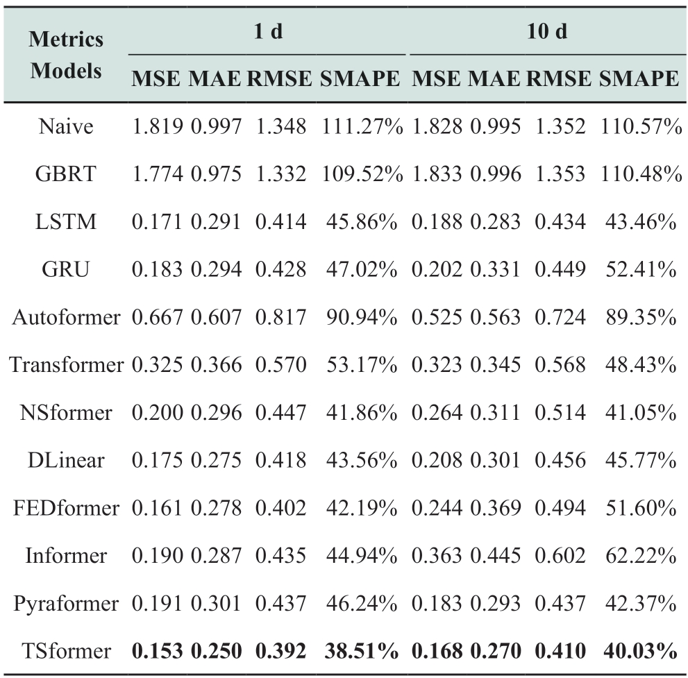
Table 3 Comparison of model performance on Solibro dataset

2.2 Experimental setup

The experimental environment was constructed using a 14 vCPU Intel(R) Xeon(R) Gold 6330 CPU @ 2.00GHz processor,RTX 4090 (24 GB) graphics card,and PyTorch 1.10.The two-stage PV power prediction model,namely TSformer,was constructed using an inverted transformer backbone,a weighted series decomposition unit,and ProbSparse attention.During the training process,the batch size,initial learning rate,number of attention heads,and dimensionality of the hidden states were set to 64,0.001,eight,and 512,respectively.MSE was used as the loss function,and Adam was used as the optimizer.The data were divided into training,validation,and test sets in a 7:1:2 ratio,and 96 past time steps were used to predict the future PV power.

2.3 Evaluation Metrics

Mean absolute error (MAE),mean square error (MSE),root mean square error (RMSE) and symmetric mean absolute percentage error (SMAPE) were used to evaluate and improve the model.Smaller values of MAE,MSE,RMSE,and SMAPE indicate better prediction accuracy.

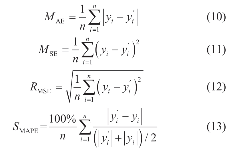
Here,n is the number of samples,yi is the true value,and is the predicted value.

2.4 Experimental Results

2.4.1 Model performance evaluation

Based on the model parameter settings mentioned in Section 3.2,we conducted performance comparison experiments of different models based on the Sanyo and Solibro power plant datasets to compare the performances of different models in PV power prediction tasks.Tables 2 and 3 present the prediction performance for the Sanyo and Solibro power station datasets,respectively.Based on the tables,the proposed model exhibits excellent prediction performance with different prediction steps for both datasets.The main focus is on the short-and medium-term forecasting performance.For convenience of representation,d is used to denote days.

(1) Short-mid term results evaluation on Sanyo

The Naive model assumes that future power values are equal to the current values,whereas the GBRT model is a gradient-augmented regression tree model.According to the experimental results,the Naive and GBRT models performed poorly in predicting the future PV power,with MSE values of 1.819 (1 day) and 1.828 (10 days) on the Sanyo dataset.This is a poorer prediction performance compared to other models,caused by the inability of this model to extract sequential complex nonlinearity.The GBRT lacks the ability to extract the temporal sequentially of PV data;therefore,the prediction performance is poor.

LSTM and GRU can extract the time dependence in the PV series and thus achieve good performance.LSTM has an MSE of 0.171 when predicting one day in the future on the Sanyo dataset.Our method exhibits a 13.56% reduction in the MSE metrics compared to the LSTM.This shows that our method can learn more explicit multivariate correlations and volatilities than LSTM.Deep learning models such as transformer,informer [24],NSformer,and Pyraformer performed well owing to their ability to extract nonlinear features and long-term dependencies in the sequences.While TSformer was able to capture the multivariate feature correlation of the PV data while extracting the long-term dependencies,the MSE,MAE,and RMSE metrics on the Sanyo dataset were reduced by approximately 52.92%,31.69%,and 31.23% (1 day),respectively,compared to those of the transformer (47.99%,21.74%,and 27.82% (10 days),respectively).The Pyraformer exhibited reduction in MSE of 19.90% (1 day) and 8.20% (10 days).The DLinear[25] and Autoformer [26] models consider the periodicity,seasonality,and other characteristics of the time series.DLinear has RMSE values of 0.418 (1 day) and 0.456 (10 days) on the Sanyo dataset,whereas our model improves the MSEs on the Sanyo dataset by 12.57% (1 day) and 19.23%(10 days) compared to those of DLinear.These results show that our method can not only extract the multivariate feature correlation of the PV data,but also capture sequence periodicity.

(2) Short-mid term results evaluation on Solibro

For the Solibro dataset,the TSformer model achieved significant performance benefits.When predicting one day into the future,the MSE,MAE,and RMSE were reduced by 5.58%,9.06%,and 31.23%,respectively,compared to those of the transformer.When predicting 10 days into the future,the MSE values improved by 56.29%,67.36%,47.48%,and 43.44% compared to those of FEDformer [27],DLinear,Informer,and Pyraformer,respectively.The performance on both datasets proves that our model has a good predictive performance.

(3) Results visualization and comparison

Figure 4 shows the comparison of four metrics of four models on two datasets,namely (a) MAE,(b) MSE,(c)RMSE,and (d) SMAPE,where red and blue indicate the prediction of one day and ten days power,respectively,in the future for the Sanyo dataset,and green and purple color indicate the prediction of one day and ten days power,respectively,in the future for the Solibro dataset.As shown in the figure,the model proposed in this paper achieves significant performance advantages on both the Sanyo power plant and Solibro power plant datasets and has an obvious advantage over other models in terms of prediction accuracy.This indicates that our method can extract the complex nonlinearity,multivariate feature correlation,and periodicity of PV data.Therefore,it has better prediction performance and generalization ability.

Figs.5 and 6 show the forecasting results for one day and ten days,respectively.The results of the TSformer model were closer to the true values and outperformed the other models in terms of accuracy,demonstrating the effectiveness of our approach in capturing the underlying patterns and dynamics of photovoltaic power generation.The improvement of the TSformer model was particularly evident in multi-step and long-term forecasting,where the complexity and uncertainty of the PV power make accurate predictions more challenging.

2.4.2 Computational efficiency analysis

To explore other performance metrics of the model,we set the batch size to 128 and analyzed the MACs,memory,and time of the model during the training process using the thop and PyTorch libraries.MAC denotes the number of multiplicative and additive operations,that is,the computational complexity of the model.The higher the MAC,the higher the computational complexity of the model.Memory indicates the memory footprint during model training;the higher the memory footprint,the higher the device memory required for model training.Time indicates the model training time;the shorter the time,the lesser the training time required by the model.These metrics determine the hardware device and time overhead required by the model during training.

The differences between full and ProbSparse attention were first compared and analyzed.As shown in Fig.7,both full and ProbSparse attention exhibited growing trends in MACs,memory,and time as the prediction length increased.However,ProbSparse exhibited a higher time efficiency under the same conditions,and the growth in MACs and memory was relatively small.When predicting the next 10 days,the latter improves by 2.28%,29.43%,and 26.94% in terms of MACs,memory,and time,respectively,over the former;thus,ProbSparse attention can achieve better performance when dealing with PV data with a longer time span.

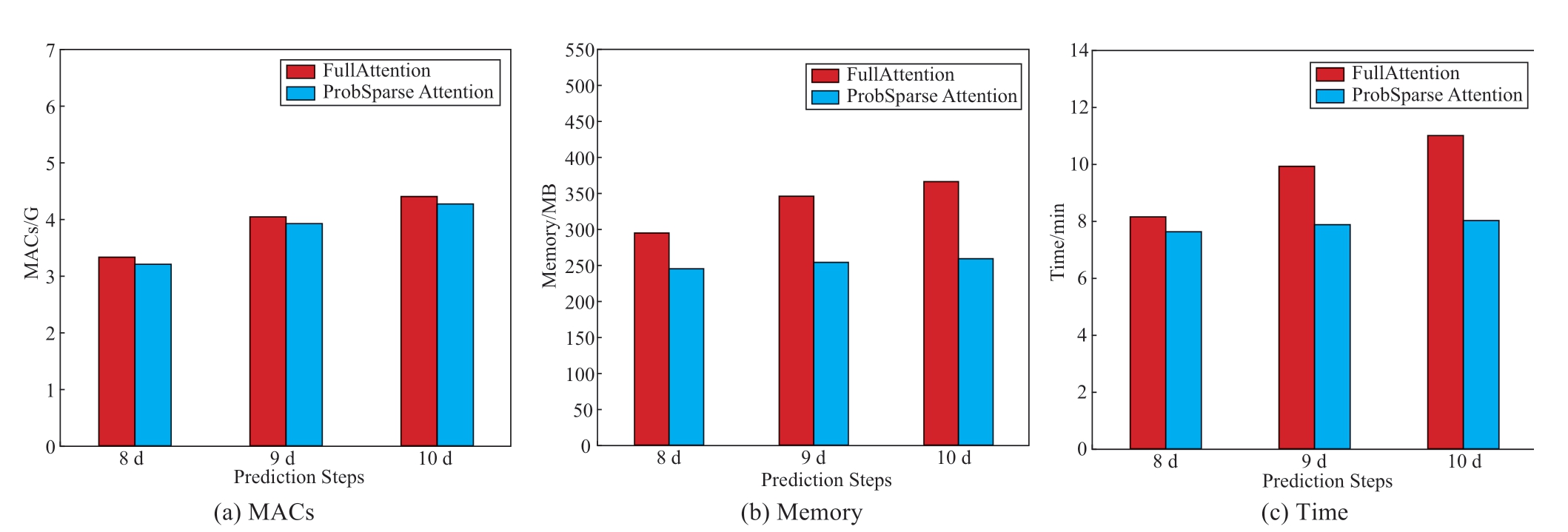
Fig.7 Classical attention vs.sparse attention

The computational complexity of the model training phase,memory consumption,and training time are listed in Table 4.TSformer is analyzed in comparison with the transformer and its variant models autoformer,NSformer,informer,Pyraformer,and FEDformer.The MACs and memory of all the models showed a gradual increase as the output length increased.However,TSformer consistently showed lower computation in terms of the MACs.Compared with the transformer,memory occupancy was reduced by 58.58% (1 day),61.34% (3 days),65.18% (5 days),and 68.69% (7 days),respectively.When the prediction time exceeded nine days the transformer and NSformer models required higher memory,leading to the problem of not being able to be trained due to insufficient memory,as shown by“Nan” in Table 4.In terms of time,TSformer achieved the best results,significantly outperforming the other models.As shown in Fig.8,the proposed model exhibited excellent performance and computational efficiency for all metrics,indicating that TSformer is more efficient when dealing with data of different prediction lengths.

Table 4 Comparison of model computational efficiency

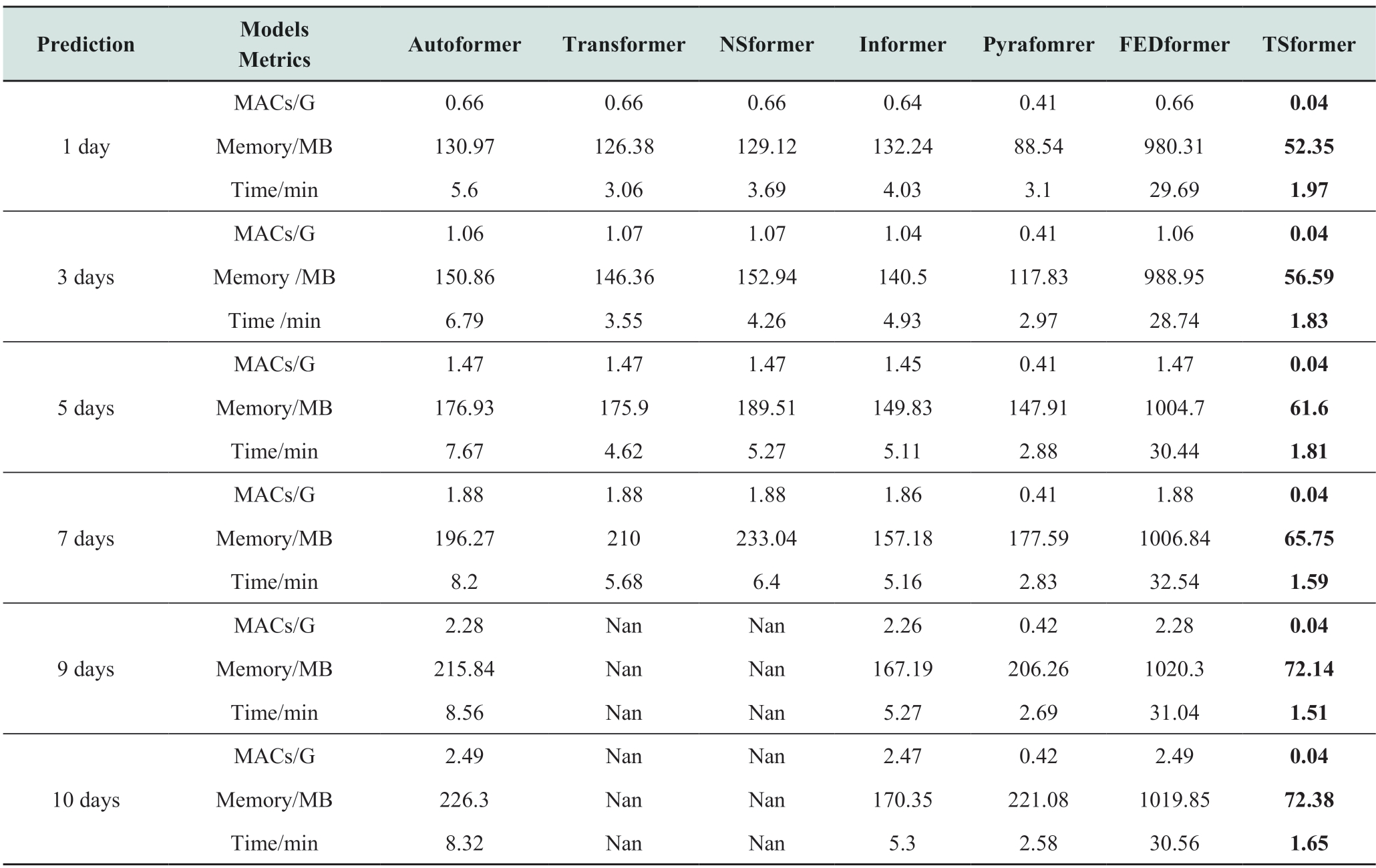
Fig.8 Model efficiency charts

In summary,compared with the baseline model,TSformer shows better performance in terms of computation,memory occupation,and processing time.This indicates that the model proposed in this paper can effectively reduce memory occupation and improve the computational efficiency of the model.

2.4.3 Analysis of ablation experiments

This subsection creates five TSformer-based variants of the model and compares TSformer with these variants to understand the impact of the many modules of TSformer on the prediction performance.The differences between the model variants are described below.

(1) No ALL: This model removes all improvement modules from TSformer,that is,the original transformer is used for the prediction.

(2) No Invert: This model removes the inverted transformer backbone from TSformer.

(3) No problem: The model uses a common attention mechanism instead of ProbSparse attention.

(4) No Sin: This model removes the Weighting Mechanism constructed on the sin function from TSformer.

(5) No Decomp: The series decomp module is removed from the TSformer.

As shown in Table 5,on the Sanyo dataset,TSformer improves the MAE compared to no ALL,no Invert,no Prob,no Sin,and no Decomp in predicting the PV power for the next five days by about 16.84%,23.42%,9.70%,3.20%,and 1.63%,respectively;and the RMSE improves by about 20.77%,14.69%,5.12%,1.77%,and 1.27% respectively.TSformer has the largest improvement compared to no ALL,which indicates that the performance improvement is obvious after introducing all the modules proposed in this paper.TSformer has a larger improvement in prediction performance compared to no Invert after removing a single module.This result proves that an invert transformer backbone can help the TSformer to improve the prediction performance significantly.

Table 5 Results of ablation experiments

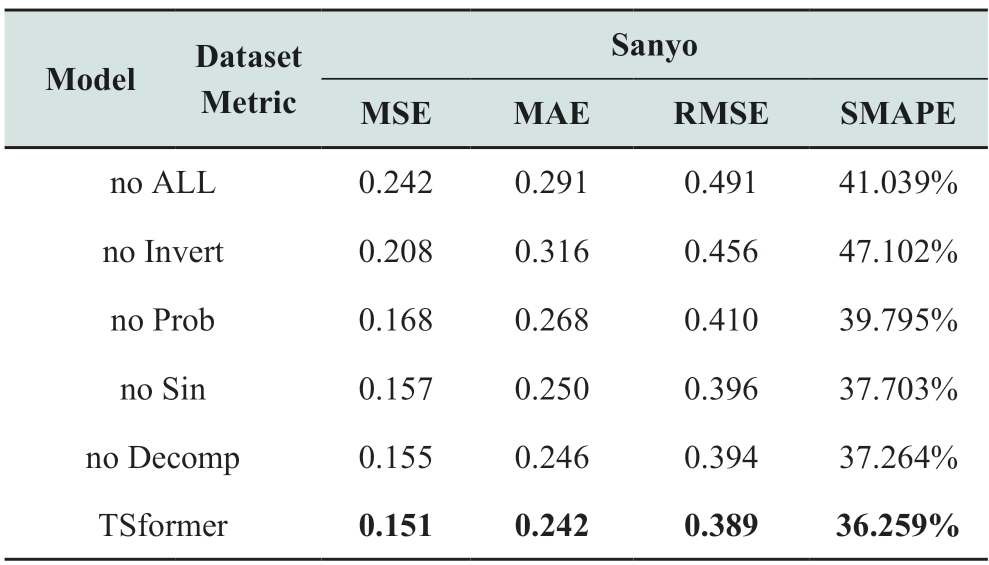
The results of the ablation experiments are visualized and analyzed to better explain the performance of the TSformer model.Based on the results in Fig.9,TSformer consistently shows significant advantages in terms of the MSE,MAE,RMSE,and SMAPE metrics.The performance improvement of TSformer compared with no inversion is relatively significant,indicating that the inverted transformer backbone plays an important role in inverting transformer backbones.Inverted transformer backbones can better model the characteristics between different variables in PV data through the duties of inverted attention and feedforward neural networks,thereby improving the accuracy of the PV prediction.Meanwhile,no Invert is slightly worse than no ALL in terms of MAE and SMAPE indicators,whereas the individual ablation model enhancement after the introduction of the inverted transformer backbone is more stable,indicating that inverted transformer backbones not only improve the prediction accuracy but also enhance model stability.Under the MSE metric,TSformer improved by approximately 10.12%,3.82%,and 2.58% compared with no Prob,no Sin,and no Decomp,respectively.This indicates that ProbSparse attention can enhance the ability of the model to extract long-range dependencies,and the weighting mechanism and weighted series decomposition units constructed based on the PV physical constraints and sine function can extract the cyclic characteristics of the PV data,further improving the accuracy of the PV power prediction.The TSformer model significantly outperforms the no Prob,no Sin,and no Decomp models in PV power prediction.The performance of the TSformer model in PV power prediction was significantly better than those of no ALL,no Invert,no Prob,no Sin,and no Decomp,highlighting the effectiveness of the inverted transformer backbone,ProbSparse attention,and weighted series decomposition module constructed by considering physical constraints in capturing the complex nonlinear,multivariate correlation,and periodicity of PV data.

3 Conclusion

Accurate PV forecasting is crucial for the development of the PV industry.This study analyzes the factors affecting the PV performance and proposes a two-stage prediction model using an optimized transformer.The use of ProbSparse attention reduces the memory occupation of the model and improves the computational efficiency of the model;the introduction of the invert transformer backbone,which inverts the duties of ProbSparse attention and FFN,allows the model to focus on the multivariate correlation of the characteristics of the PV power series and capture the series non-linearity and volatility.To extract the periodic characteristics of the PV power sequence,a weighted-series decomposition module combining the PV characteristics was proposed to constrain the output of the model to fit the periodic characteristics of the original sequence.The final prediction results were obtained using additive reconstruction.The model performance was validated using the Sanyo and Solibro power station datasets.The results showed that the model exhibits improved prediction accuracy and computational efficiency compared with the transformer and baseline models.Deep learning models should be data driven and incorporate domain knowledge to guide their construction and training.The two-stage model proposed in this study to optimize the transformer takes advantage of the photovoltaic domain change features for improvement.The first stage combines the characteristics of the PV power data to optimize the transformer model,and the second stage considers the characteristics of the PV power cycle and combines the advantages of the two stages to improve the prediction accuracy,robustness,and computational efficiency of the model.The construction process of this method demonstrates that it is necessary and meaningful to consider the physical characteristics of a specific engineering problem when constructing deep-learning models.This knowledge can help the model obtain better accuracy and robustness and improve the computational efficiency.

Future work should incorporate additional physical laws and expert knowledge in the PV field to further enhance the PV forecasting performance.

Acknowledgments

This work was supported by Top Leading Talents Project of Gansu Province(B32722246002).

Declaration of Competing Interest

We declare that we have no conflict of interest.

References

[1] Bai M,Zhou Z,Chen Y,et al.(2023) Accurate four-hour-ahead probabilistic forecast of photovoltaic power generation based on multiple meteorological variables-aided intelligent optimization of numeric weather prediction data.Earth Science Informatics,16(3): 2741-2766

[2] Belmahdi B,Louzazni M,Bouardi A E.(2020) A hybrid ARIMA-ANN method to forecast daily global solar radiation in three different cities in Morocco.The European Physical Journal Plus,135: 1-23

[3] Jeong H Y,Hong S H,Jeon J S,et al.(2022) A Research of Prediction of Photovoltaic Power using SARIMA Model.Journal of Korea Multimedia Society,25(1): 82-91

[4] Banik R,Biswas A.(2023) Improving Solar PV Prediction Performance with RF-CatBoost Ensemble: A Robust and Complementary Approach.Renewable Energy Focus,46: 207-221

[5] Ramos L,Colnago M,Casaca W.(2022) name="ref6" style="font-size: 1em; text-align: justify; text-indent: 2em; line-height: 1.8em; margin: 0.5em 0em;">[6] Alrashidi M,Rahman S.(2023) Short-term photovoltaic power production forecasting based on novel hybrid name="ref7" style="font-size: 1em; text-align: justify; text-indent: 2em; line-height: 1.8em; margin: 0.5em 0em;">[7] Ma X Y,Zhang X H.(2022)A short-term prediction model to forecast power of photovoltaic based on MFA-Elman[J].Energy Reports,8: 495-507

[8] Sharma J,Soni S,Paliwal P,et al.(2022) A novel long term solar photovoltaic power forecasting approach using LSTM with Nadam optimizer: A case study of India.Energy Science &Engineering,10(8): 2909-2929

[9] Sarkar S,Karthick A,Kumar Chinnaiyan V,et al.(2023) Energy forecasting of the building-integrated photovoltaic façade using hybrid LSTM.Environmental Science and Pollution Research,30(16): 45977-45985

[10] Li Z,Xu R,Luo X,et al.(2022) Short-term photovoltaic power prediction based on modal reconstruction and hybrid deep learning model.Energy Reports,8: 9919-9932

[11] Kothona D,Panapakidis I P,Christoforidis G C.(2022) A novel hybrid ensemble LSTM-FFNN forecasting model for very shortterm and short-term PV generation forecasting.IET Renewable Power Generation,16(1): 3-18

[12] Chen H,Chang X.(2021) Photovoltaic power prediction of LSTM model based on Pearson feature selection.Energy Reports,7: 1047-1054

[13] Li Y,Ye F,Liu Z,et al.(2021) A short-term photovoltaic power generation forecast method based on LSTM.Mathematical Problems in Engineering,2021: 1-11

[14] Tian F,Fan X,Wang R,et al.(2022) A Power Forecasting Method for Ultra-Short-Term Photovoltaic Power Generation Using Transformer Model.Mathematical Problems in Engineering,2022(1): 9421400

[15] Gao Y,Miyata S,Matsunami Y,et al.(2023) Spatio-temporal interpretable neural network for solar irradiation prediction using transformer.Energy and Buildings,297: 113461

[16] Gao X,Liu J,Yuan Y,et al.(2024) Global horizontal irradiance prediction model considering the effect of aerosol optical depth based on the Informer model.Renewable Energy,220: 119671

[17] Cao Y,Liu G,Luo D,et al.(2023) Multi-timescale photovoltaic power forecasting using an improved Stacking ensemble algorithm based LSTM-Informer model.Energy,283: 128669

[18] Jiang Y,Gao T,Dai Y,et al.(2023) Very short-term residential load forecasting based on deep-autoformer.Applied Energy,328: 120120

[19] Tan F,Xu G,Li Y,et al.(2022) A method of transformer top oil temperature forecasting based on similar day and similar hour[J].Electric Power Engineering Technology,41(2): 193-200

[20] Yan J,Hu L,Zhen Z,et al.(2021) Frequency-Domain Decomposition and Deep Learning Based Solar PV Power Ultra-Short-Term Forecasting Model.IEEE Transactions on Industry Applications,57(4):3282-3295

[21] Liu X,Liu Y,Kong X,et al.(2023) Deep neural network for forecasting of photovoltaic power based on wavelet packet decomposition with similar day analysis.Energy,271:126963

[22] Zhou Y,Shi K,Li D,et al.(2023) Calculation of load aggregator potential and peak regulation strategy based on longitudinal modified ARIMA.Electric Power Engineering Technology,42(2): 2-10

[23] Luo X,Zhang D,Zhu X.(2021) Deep learning based forecasting of photovoltaic power generation by incorporating domain knowledge.Energy,225: 120240

[24] Wu R,He Y,Jiang J,et al.(2023) Temperature and pressure characteristics of dissolved acetylene in transformer oil based on photothermal interference detection system.Electric Power Engineering Technology,42(5):30-36

[25] Zeng A,Chen M,Zhang L,et al.(2023) Are transformers effective for time series forecasting?[C]//Proceedings of the AAAI conference on artificial intelligence,37(9): 11121-11128

[26] Wu H,Xu J,Wang J,et al.(2021) Autoformer: Decomposition transformers with auto-correlation for long-term series forecasting.Advances in Neural Information Processing Systems,34: 22419-22430

[27] Zhou T,Ma Z,Wen Q,et al.(2022) Fedformer: Frequency enhanced decomposed transformer for long-term series forecasting//International Conference on Machine Learning.PMLR,2022: 27268-27286

Scan for more details

Received: 28 April 2024/ Received: 18 September 2024/ Accepted: 30 September 2024/ Published: 25 December 2024

Feng Li

lifeng@llu.edu.cn

Yanhong Ma

myh_2005@163.com

Hong Zhang

zhanghong@lut.edu.cn

Guoli Fu

2822168615@qq.com

MinYi

yi_min2022@163.com

2096-5117/© 2024 Global Energy Interconnection Group Co.Ltd.Production and hosting by Elsevier B.V.on behalf of KeAi Communications Co.,Ltd.This is an open access article under the CC BY-NC-ND license (http://creativecommons.org/licenses/by-nc-nd/4.0/).

Biographies

Yanhong Ma received his bachelor’s degree in power system automation from Lanzhou University of Technology in 2001,his master's degree in control theory and control engineering systems from Lanzhou University of Technology in 2004.He is working in the State Grid Gansu Electric Power Company,Lanzhou.His research interests include artificial intelligent and smart grid.

Feng Li received his bachelor’s degree in software engineering from the Business College of Shanxi University in 2021.He is working towards master’s degree at Lanzhou University of Technology.His research interests include artificial intelligence and photovoltaic power forecasting.

Hong Zhang received bachelor’s degree in computer science and technology from Lanzhou University of Technology in 2001,master’s degree in communication and information systems from Lanzhou University of Technology in 2004,Ph.D.in system engineering from Lanzhou University of Technology in 2018.She is working at Lanzhou University of Technology.Her research interests include artificial intelligent and data analysis.

Guoli Fu received his bachelor’s degree in electrical engineering and automation from Henan University of Engineering in 2021.He is working towards master’s degree at Lanzhou University of Technology.His research interests are artificial intelligence and photovoltaic power forecasting.

Min Yi received her bachelor’s degree in information and computational science from Lanzhou University of Technology in 2022.She is working towards master’s degree at Lanzhou University of Technology.Her research interests are artificial intelligence and traffic flow forecasting.

(Editor Yu Zhang)