0 Introduction
The rapid current rise in clean energy has become a critical step towards the sustainable development of renewable energy [1].According to data from China Wind Power Lifting Capacity Statistical Brief, by the end of 2022,the number of wind turbines (WTs) exceeds 180000, whose total installed capacity also exceeds 390 million kilowatts,which is 14.1% more than that of the previous year [2].With the increasing progress and large-scale application of wind power technology, managing and processing the massive amounts of data generated by wind farms to guarantee the accuracy of wind farm optimization control and power prediction has become an important issue in current research [3].
An enormous amount of data from the Supervisory Control and Data Acquisition (SCADA) systems of wind turbines contains several outliers, including missing,constant, and overlimit values, which are influenced by the surroundings and measuring equipment.Cleaning is necessary for practical modeling because the use of unprocessed data might result in an anomalous curvature of the wind power curve (WPC), which impairs the accuracy of the power curve modeling and power forecast findings [4].
There are two main types of traditional wind power anomaly data identification and cleaning methods.The first type is a statistical feature-based method that analyzes statistical features, including variance, data density, and data point spacing, to identify wind power anomaly data.In Ref.[5], a method combining boundary extraction and boundary regularization was proposed.For stacked anomalies in the wind power curve, the density difference between the normal and outlier points in the data is fully utilized to obtain better cleaning performance.However,the improved density clustering algorithm affects the final anomalous data identification and cleaning effect if the clustering center is not properly selected.The performance of the boundary extraction algorithm is largely dependent on the characteristics of the data distribution, which needs to be verified in more power generation scenarios.In Ref.[6], a clustering algorithm based on DBSCAN density was proposed, combined with the Laida criterion, which could effectively filter out the anomaly discrete data.Although this method can efficiently recognize discrete data under faulty conditions, the sample data, which are divided into several segments by the intervals of wind speed and processed, lose the global data features and does not validate the effectiveness of identifying horizontal stacking anomaly data.In Ref.[7], a multivariate outlier identification method based on the Mahalanobis distance and k-means clustering was proposed.However, the limited number of data observations can affect the ability of the algorithm to identify anomalous data when observing data in different power-generating scenarios, leading to classification anomalies.In Ref.[8], the Thompson tau-quartile method was used to segment the anomalous operational data by dividing the wind speed intervals for refined cleaning.Nevertheless, the algorithm may misclassify or overlook genuine anomalies in instances where the data exhibit bimodal or skewed distributions.Based on the above references, it is evident that statistical attribute-based algorithms used in multifeatured wind power anomaly data recognition may struggle to precisely capture these intricate patterns, thereby diminishing the efficacy of abnormal data cleaning.
The second type is based on the mathematical modeling of wind power curves; scholars have extensively studied various mathematical modeling methods, including parametric and non-parametric models.After modeling, the data outside the model boundary are regarded as anomalies with the aim of accurately defining the boundary between normal and abnormal data to improve the accuracy of data cleaning [9].In Ref.[10], a variable bin width method was proposed to categorize wind speed data into bins of different intervals, with the aim of determining the average power output for each ordered bin; cubic B-spline interpolation was concurrently employed to accurately fit the power curve.This methodology allows for the determination of the power output range for each turbine unit by calculating the standard deviation within each wind speed bin, identifying any data points that fall outside the predefined upper and lower limits as outliers.Nevertheless, the efficacy of the variable bin width approach is contingent on the availability of a substantial volume of data to ensure the accurate calculation of the mean and standard deviation within each bin.Under conditions where data are sparse or the distribution of wind speeds is uneven, statistical calculations may become unstable, which can adversely affect the establishment of upper and lower limits and the identification of outlier data.
Unlike parametric modeling methods, non-parametric modeling does not assume that the data follow any specific functional form or distribution; instead, it models based on the inherent characteristics of the data, thereby enhancing its capability to capture nonlinear relationships and patterns[9].Ref.[11] proposed a heterogeneous stacked regressor(HET-SR) model that employs locally estimated scatterplot smoothing (LOESS) for a robust estimation to obtain the power curve.Using the trained HET-SR model, potential outliers were identified to compare the differences between the actual and model-predicted power outputs.However,this model integrates multiple distinct regression algorithms and achieves model fusion through a stacking approach,resulting in a complex structure and high training cost.In Ref.[12], an anomaly data identification algorithm based on adaptive confidence boundary modeling (ACBM) was proposed.This method uses an expectation-maximization algorithm to estimate a weighted mixture of Archimedes’copula functions, thereby establishing a joint probability distribution.It further incorporates a confidence boundary modeling approach for the power curve to identify anomalous data.However, this approach is highly dependent on the quality of the original SCADA data; systematic biases or errors during data collection can propagate through the preprocessing stage to the final model, thereby affecting its accuracy and reliability.
In recent years, with the progressive deepening of research in computer science and data science, a plethora of new technologies has emerged in the direction of anomaly detection for wind power data.In Ref.[13], a deep learning model that integrates stacked denoising autoencoders(SDAE) with a density grid-based clustering method was proposed to detect anomalies in wind power data.However,configuring hyperparameters such as hidden layers and learning rates for the SDAE model requires substantial time and computational resources for training and optimization; failure to configure these parameters properly can adversely affect the final data cleaning efficacy.In Ref.[14], a composite machine learning algorithm based on the horizontal and vertical quartile method combined with an extreme learning machine (ELM) was proposed for identifying anomalies in wind speed-power data within wind farms.However, the computational cost and execution efficiency of the algorithm, which are critical considerations for resource-constrained environments or application scenarios that require a rapid response, have not been discussed.In Ref.[15], a method was proposed that transforms data cleaning issues into image segmentation problems by image thresholding based on the minimization of dissimilarity-and-uncertainty-based energy (MDUE),thereby effectively identifying and cleaning abnormal data.However, when processing large datasets, this approach involves converting a vast number of data points into digital images and undertaking complex image-processing steps,resulting in reduced computational efficiency.In Ref.[16], a wind farm abnormal operational data cleaning method based on segmented image recognition was proposed.This method employs a dispersed anomaly pixel identification model based on Canny edge detection and a stacked anomalous pixel point recognition model based on mathematical morphology to facilitate the cleaning of abnormal data.However, this method also requires the consideration of the overall structure and relationships between wind power data to achieve a more refined identification of horizontally stacked anomalous data.
In summary, current strategies for identifying and cleaning anomalous wind power data have drawbacks.Statistical feature-based methods can misidentify stacked anomalous data in the middle of the curve as normal data because of their high density and similar distance characteristics, resulting in lower identification accuracy.Methods based on wind power curve modeling are highly dependent on the quality of the data used for modeling: if the input data contain a significant amount of noise or errors, it can lead to decreased model accuracy and affect the effectiveness of data cleaning.Methods based on composite machine learning algorithms must carefully consider the algorithm’s parameter configuration, computational cost, and execution efficiency in different environments.Direct image processing recognition methods rely solely on the local features of images,such as edges, colors, and textures, making it difficult to capture the global structure and complex relationships of the wind power curve, leading to poor recognition performance in style="font-size: 1em; text-align: justify; text-indent: 2em; line-height: 1.8em; margin: 0.5em 0em;">Section 1 of this paper shows the cleaning process of the CWPAD-IPCDA method.Section 2 describes the preprocessing of each dataset.Section 3 describes the undirected graph construction method and the Louvain community discovery algorithm for wind power data and analyzes the initial cleaning effect of anomalous data under the combination of parameters and determines the main part of WPC image with the help of mathematical morphology operations to complete the final anomaly data cleaning.Section 4 compares and analyzes the simulation experimental results of the four anomaly data cleaning algorithms on each dataset and verifies the better cleaning performance of the CWPAD-IPCDA method.
1 CWPAD-IPCDA cleaning process
Owing to environmental factors and the impact of the equipment itself, WTs in the actual operation process exhibit a variety of abnormal data patterns, which can be categorized into three main types [17], as shown in Fig.1.
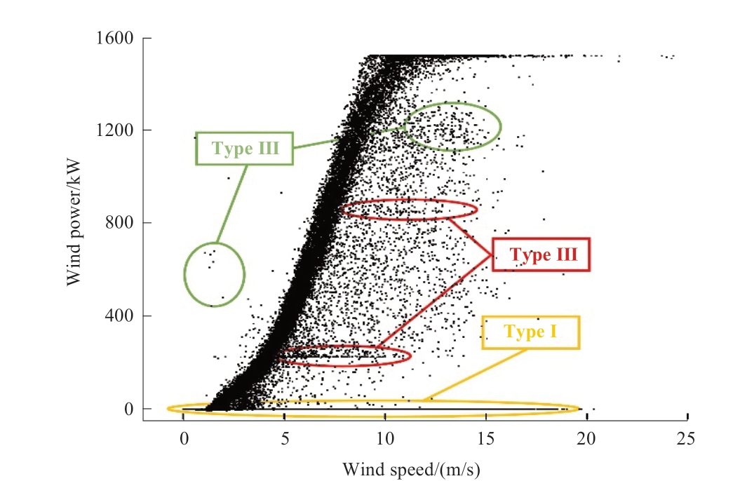
Fig.1 WPC abnormal data types based on G-01 wind turbine
The first type (Type I) is the anomalous data referring to shutdown points where the output power of wind turbines exhibits negative or near-zero values, typically due to malfunctions or maintenance activities.The second type (Type II) is the level-stacked anomalous data owing to the wind abandonment and limitation of power as well as communication failure.The third type (Type III) is the outlying anomalous data due to severe weather or the failure of equipment sensors.
The three stages of the CWPAD-IPCDA method include data preprocessing, anomalous data detection and initial cleaning, and extraction of the main part from the WPC image.To ensure the accuracy and efficacy of the subsequent steps, the first step involves manually preprocessing the data from the WTs supplied by the SCADA system which includes aberrant values beyond the normal operating range of the turbine (e.g.,Type I) and missing values.The second stage involves transforming the WPC image that has been cleared of Type I into an undirected graph structure under the proposed node and boundary construction method, optimizing the modularity of the graph using the Louvain algorithm to achieve community detection and delineation of the graph, and combining the data processing method of the node degrees and delineated communities in the graph theories to perform the initial cleaning of the abnormal nodes (Types II and III) in the undirected graph.The third stage uses the open operation in MMO to further smooth the edge contour of the WPC image and refine the noise (Type III) to obtain a more representative subject image.Finally, the optimized WPC main part is remapped back to the normal wind power points to complete the final anomaly data cleaning; the specific cleaning steps are shown in Fig.2.
The CWPAD-IPCDA method is elaborated upon in the following sections in conjunction with SCADA datasets comprising 25 WTs across two wind farms in Northwest China.
2 Data preprocessing
Aiming at the obvious missing values and Type I abnormal data in each dataset through reasonable manual preprocessing can reduce the complexity of cleaning abnormal data while ensuring the accuracy of subsequent algorithms.
The power output characteristics of a wind turbine under normal operating conditions vary according to the different input wind speeds.This relationship is expressed as follows [8]:
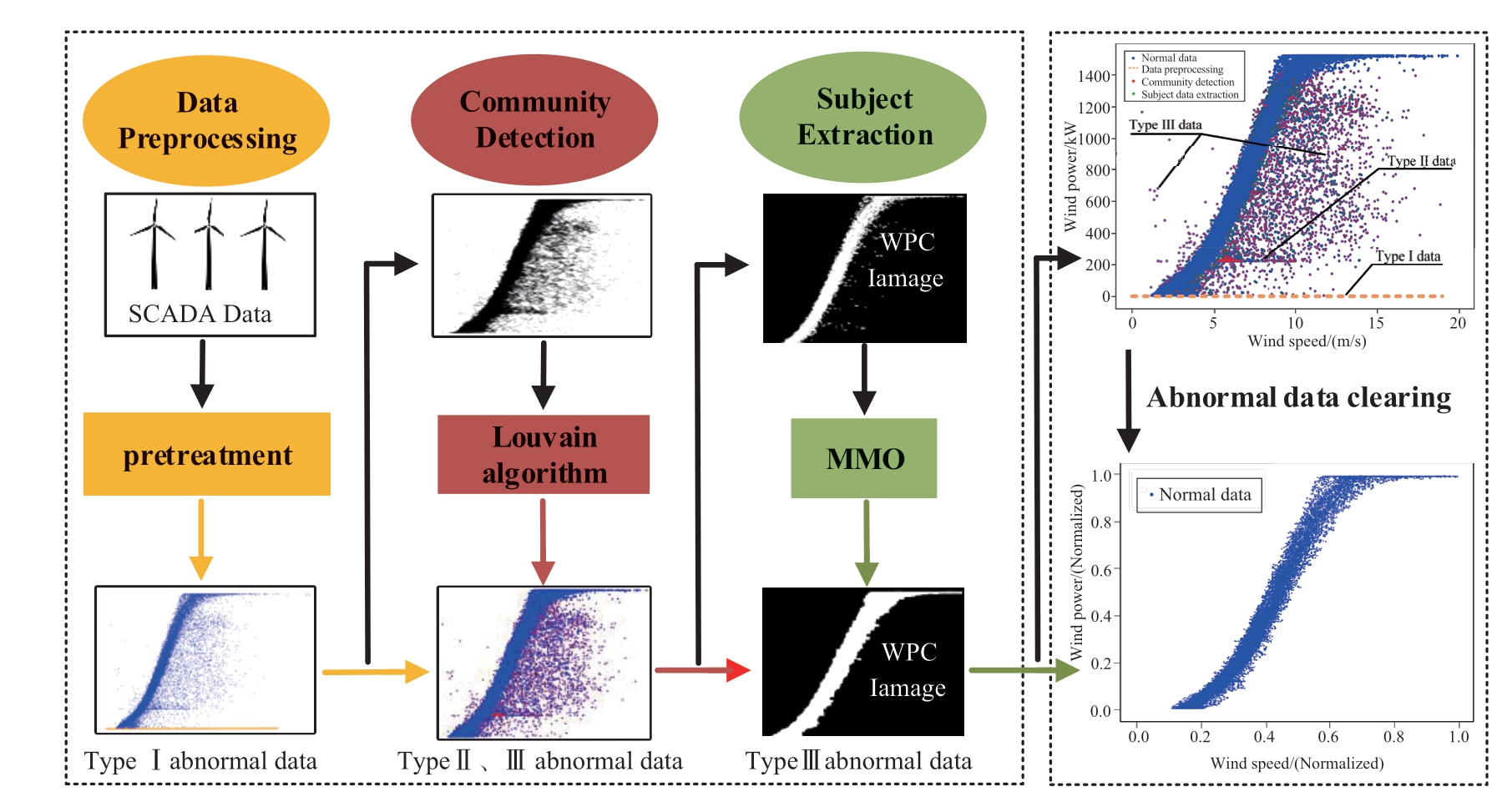
Fig.2 CWPAD-IPCDA method steps

In Eq.(1), Vc represents the cut-in wind speed, Vr the rated wind speed, Vs the cut-out wind speed, P(V) the variable power between the cut-in and rated wind speeds,and PN the rated power.
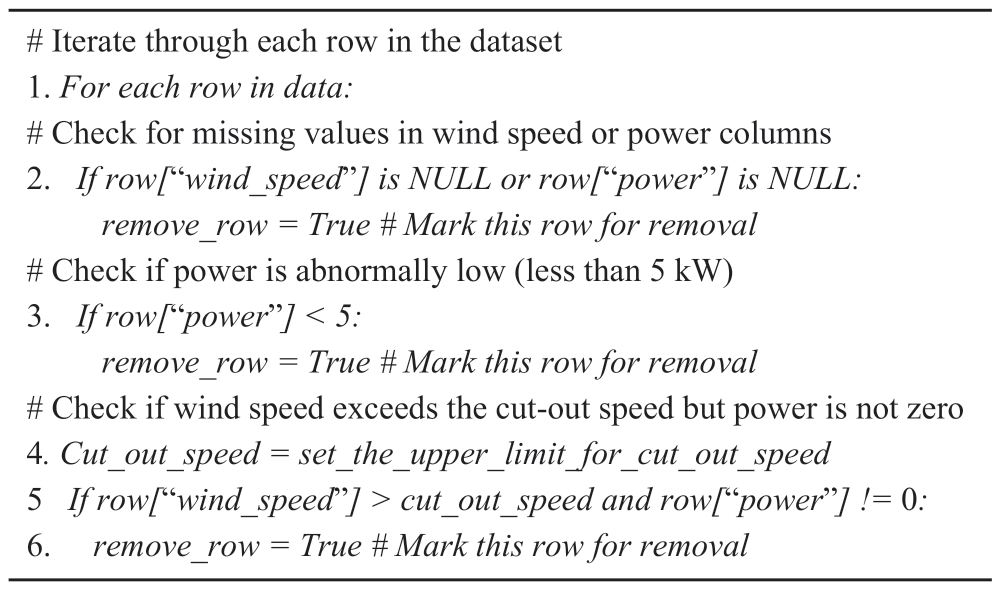
The purpose of cleaning the anomalous wind power data is to preserve the data of normal operation and remove the other three categories of anomalous data.According to Eq.(1), when the wind speed is between Vc and Vs, the power should range from P(V) to PN and should not approximate zero or be negative.Thus, the selection of Type I shutdown points is relatively straightforward; the power data is less than a certain threshold, typically set at 5 kW, should be removed [17].Data with nonzero power beyond the cut-out wind speed, missing values in the wind speed, and power columns should be directly marked and removed.The specific preprocessing pseudocode is shown in Table 1.
Table 1 Manual preprocessing of pseudocode
In wind farm I (G-01 wind turbine) and wind farm II (g-03 wind turbine), the red data points represent the cleaned Type I anomalous data and the non-zero anomalous data beyond the cut-out wind speed, whereas the blue data points indicate the remaining wind power data after preprocessing(as shown in Fig.3).
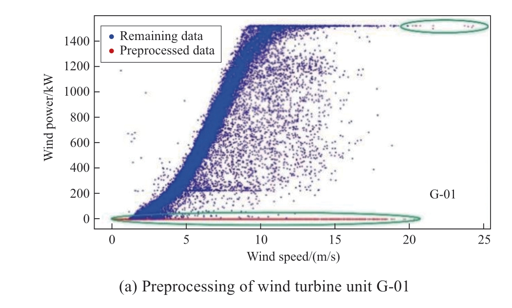
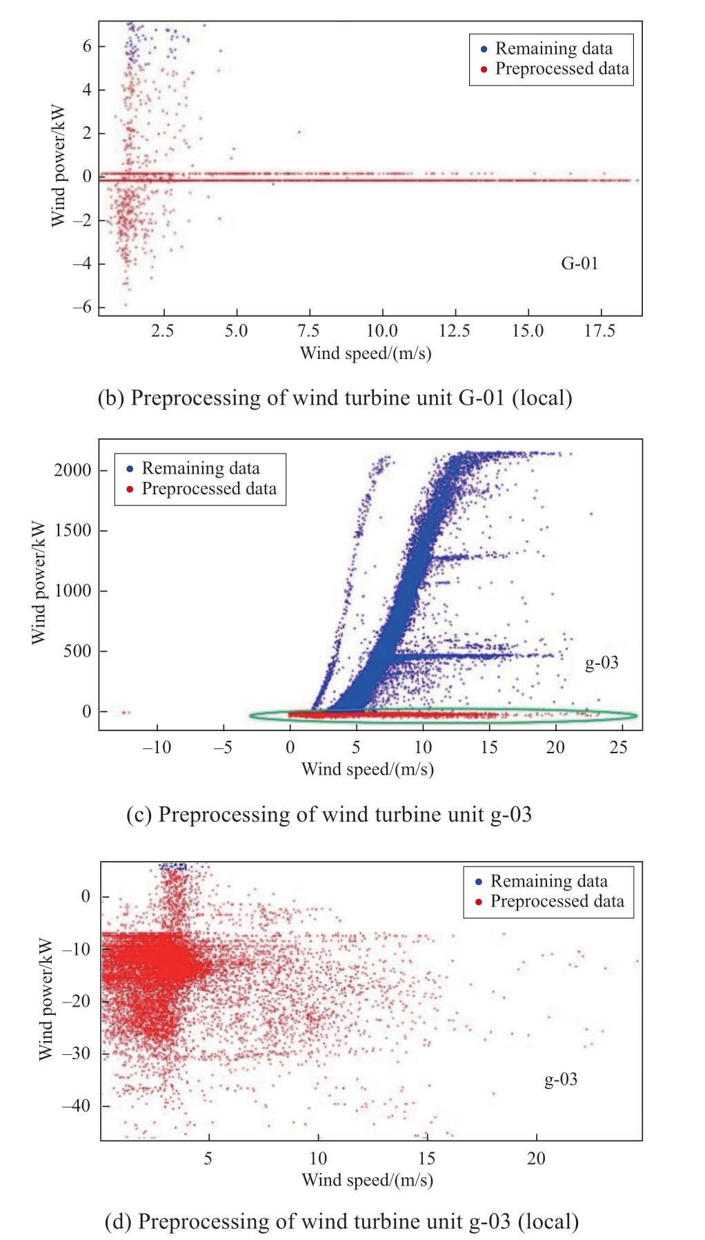
Fig.3 Preprocessing results
From subfigures (a) and (c) in Fig.3, it is evident that the shutdown points at the bottom of the wind power curves and the nonzero power outside the cut-out wind speeds for WTs G-01 and g-03 were removed.Subfigures (b) and (d) further provide a localized visualization; the negative power and near-zero anomalous data that accumulate around zero power within the normal output range of the turbines are eliminated.
3 Anomaly data detection and cleaning based on the CWPAD-IPCDA methodology
3.1 Binarization of wind power curve image
Following data preprocessing, the discrete wind speedpower data is rasterized.The resulting rasterized WPC image is denoted as f(x, y), with (x, y) standing for each pixel location.Subsequently, set the grayscale value of all pixels in f(x, y) to 0 (black).For each data point in the WPC image, set its corresponding pixel position (xi, yi) in to 255(white).
The preprocessed G-01 wind turbine WPC binarized image and local rasterized schematic are shown in Fig.4.
3.2 Undirected graph construction
According to Eq.(1), the output power of WTs follows a specific physical relationship with the wind speed.When constructing an undirected graph, this relationship is simplified into non-directional connections based on the similarity between nodes; such connections are determined by the relative positions of the data points represented by the nodes in the feature space, where closer distances indicate higher feature similarity.Simplifying the data representation in this manner facilitates the further application of community detection algorithms and graph theory methods to effectively identify anomalous wind power data.
1) Nodes establishment
The undirected graph G=(V, E), with V representing the set of nodes and E representing the set of edges, must be defined initially.Each pixel position (xi, yi) is added to the image I with a value of 255 to the node set V.Subsequently,V can be represented as

Fig.4 WPC binarized image of G-01 wind turbine
2) Establishment of the edges for nodes
Considering the spatial position information between nodes, a method for constructing boundaries based on the Euclidean distance between nodes within dynamic rectangular connection neighborhoods is proposed.The specific steps are illustrated in Fig 5.
2.1) Partitioning dynamically connected neighborhoods based on inter-node density
2.1.1) Determining the node density at the initial connection radius
The coordinate of a node Vi in the undirected graph is(i, j).D(i, j) denotes the density of this node Vi and other nodes (k, l) within the initial rectangular neighborhood connection radius r, as shown in Fig.5 (a), (b).
Where φ(k ,l ) represents the indicator function, it equals 1 if the pixel grayscale value at coordinates (k, l) in the image is 255; otherwise, it equals 0.
2.1.2) Dynamically updating the radius of connected neighborhoods based on node density
The relationships between nearby nodes may be more precisely reflected in the associations between local nodes by considering the density around the nodes and dynamically adjusting the rectangle-linked neighborhoods centered on the node Vi.The updated dynamic rectangular neighborhood connection radius R can be expressed as:
where R is the updated dynamic rectangular neighborhood connectivity radius, D' is the mean of the node densities in the undirected graph, and tanh is the hyperbolic tangent function, whose output range is [-1,1].
Using Eq.(4), the connection radius of each node can be dynamically adjusted based on the actual density D(i, j) around it.When D(i, j) is close to D', the output of the tanh function is close to 0 and R is close to r; When D(i, j)is significantly higher than D', the density around the node is high and the output of the tanh function approaches -1,and the value of 1+tanh leads to R gradually approachingzero.Oppositely, the value of 1+tanh leads R is bigger than r when D(i, j) possesses a lower valve than D', the result of the bigger R will enhance the connectivity of the lowdensity region.

Fig.5 Specific steps of the boundary construction method based on the Euclidean distance between nodes in a dynamically connected neighborhood
2.1.3) Adjusting the connection neighborhood based on the updated dynamic connection radius R
With Eqs.(3) and (4), the updated rectangular connected neighborhood N(i, j), as shown in Fig.5 (c), can be expressed as
Dynamic connection neighborhoods dynamically adjust the range of connections for each node by considering the local node density, as illustrated in section (c) of Fig.5.The fundamental principle behind this approach is to decrease the connection radius in densely populated data regions to avoid excessive connections and, conversely,to increase the radius in sparse areas to ensure network connectivity.Utilizing a nonlinear function to adjust the radius based on density allows for smoother adjustment.This enables each node to search for neighboring nodes within varying radii according to the specific circumstances of its local environment, facilitating the establishment of connections between nodes.
2.2) Introducing a nonlinear probabilistic decisionmaking mechanism for connections between nodes
A nonlinear probabilistic decision-making mechanism for connections between nodes is introduced in the updated dynamically connected neighborhoods.In other words, the connection probability between nodes Vi and Vk, which are classified as belonging to the same neighborhood, varies and decreases exponentially with increasing distance.

In Eq.(6), d(i,k) is the Euclidean distance between two nodes; in Eq.(7), P(i,k) denotes the connection probability of the two nodes, and S denotes the connection decay coefficient, determining the decay rate of the exponential decay function.
Using the edge creation method for nodes in this undirected graph, the set of edges E associated with each node Vi, Vk in N(i, j), is defined as follows:
where E represents the set of all edges in the graph, (Vi,Vk)signifies an edge between node Vi and node Vk, and θ is a randomly generated number from a uniform distribution ranging between (0, 1).
The visualization model of the edges between nodes established based on the proposed method of constructing boundaries by considering the Euclidean distance between nodes within dynamic rectangular connection neighborhoods is illustrated in Fig.5 (d).
To more accurately represent the anomalous structure present in the graph and increase the algorithm’s capacity for generalization, this section considers the nonlinear spatial location information between nodes in the undirected graph.The random number θ is introduced for comparison with the connection probability function P(i,k), which establishes the connection of edges based on probability.
Fig.6 illustrates the structure of the undirected graph of the method for building node edges based on the dynamic neighborhood and nonlinear decision mechanisms, using the G-01 wind turbine as an example.
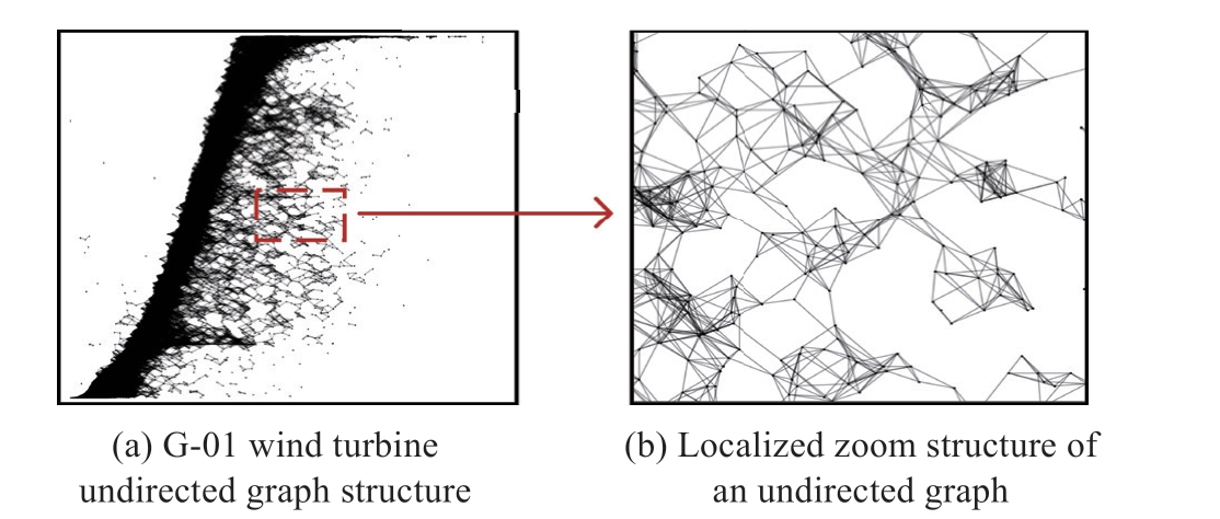
Fig.6 G-01 wind turbine global and local structure of wind turbine undirected diagrams
3.3 Community detection
The Louvain algorithm can partition a set of nodes V into several disjoint subsets C1,C2,…,Ck, each of which Ci is called a community.E is the connecting relationship between communities.The connections between nodes within each community are denser,, whereas the connections between communities are sparser.Under the detection and delineation of the Louvain algorithm, Type II powerlimited anomalies and Type III outlier anomalies behave as subcommunities that are either separate or uncorrelated with the main communities in the constructed undirected graph G (illustrated in Fig.6).The results of local delineation are presented in Fig.7.
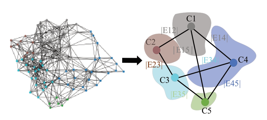
Fig.7 Localized communities delineation for G-01 wind turbine
The Louvain algorithm is a greedy algorithm that attempts to assign nodes to communities by maximizing the connection weights within communities and minimizing the connection weights between communities through local and global optimizations to obtain maximum modularity when optimizing the community partitioning of the graph [18].The modularity is expressed as follows [19]
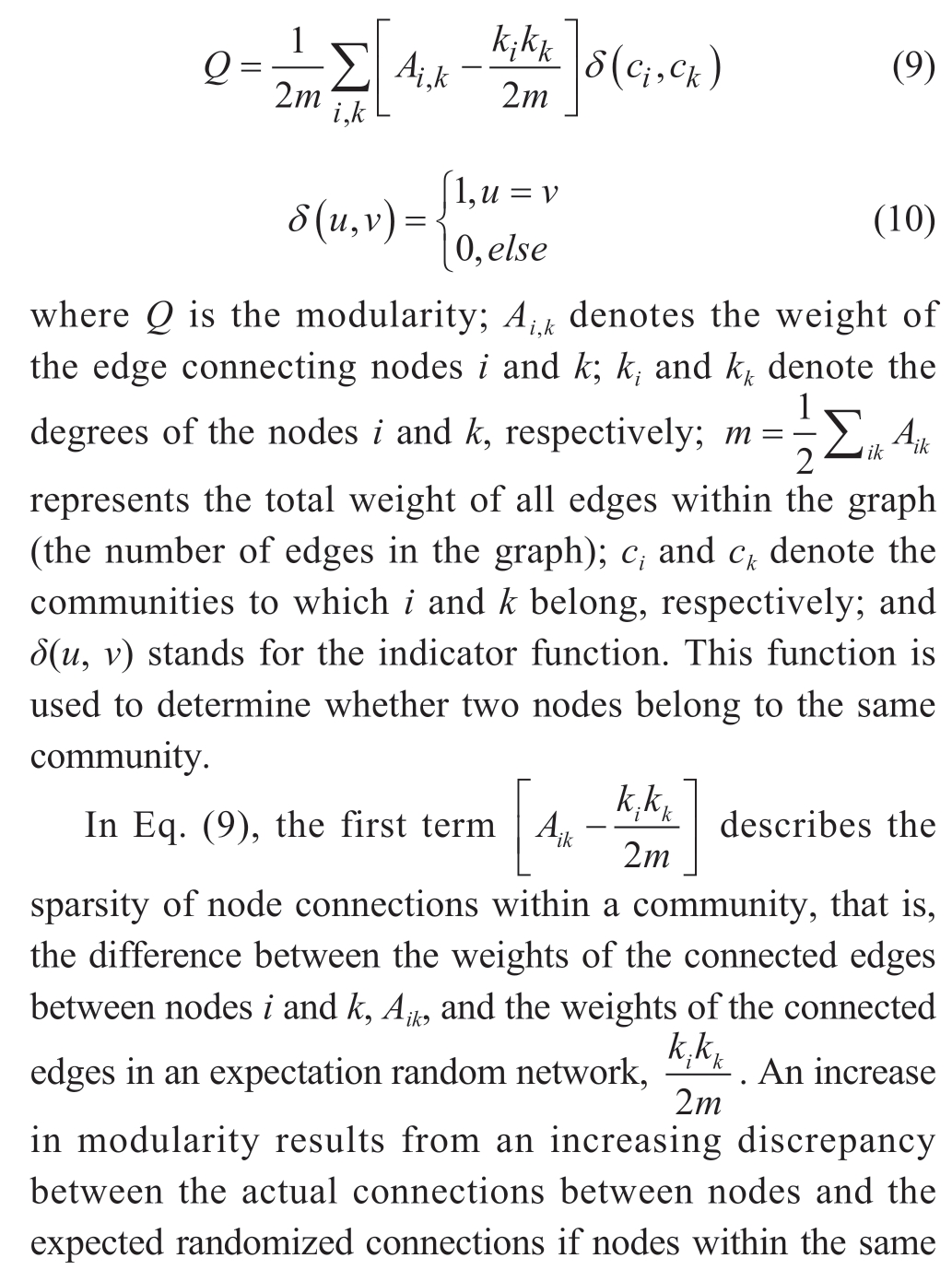

By quantifying the assignment of node communities and connections inside and outside the communities, the modularity Q reflects the sparsity of connections and the difference in connection density inside and outside the communities.The higher the modularity, the more the detected community adheres to the requirements of “inner tightness and outer looseness,” and the higher the quality of the grouping.
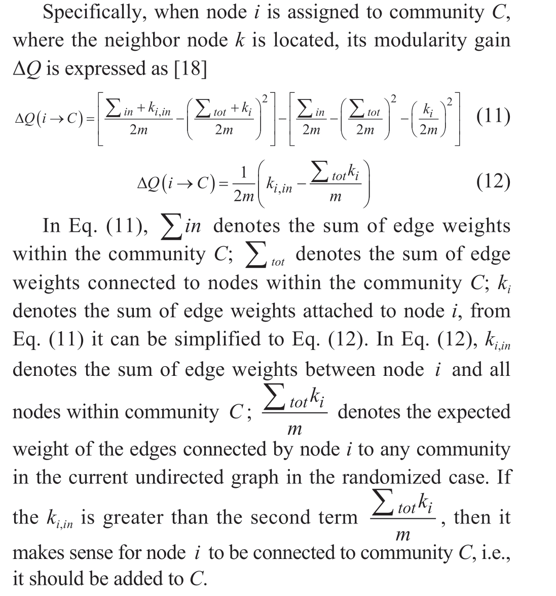
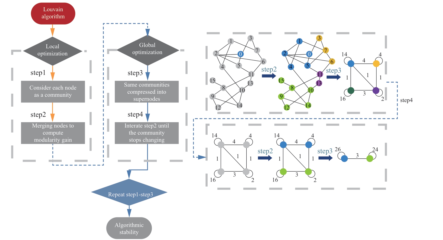
Fig.8 Louvain algorithmic process
Based on the above analysis, the Louvain community detection algorithm (shown in Fig.8) is used to provide a concrete introduction, which is divided into two phases:local and global optimization.
Local optimization considers each node of the undirected graph in Section 3.2 as a separate community,thus obtaining an initial community with the same number of nodes.Then, for each node i, community allocation is attempted by examining its relationship with the community of each neighbor node k.The change in local modularity ΔQ before and after allocation is calculated.If ΔQ is greater than zero, the node i is assigned to the community in which the neighbor node with the largest ΔQ is located; otherwise,it remains unchanged.
Global optimization entails compressing the community where node i resides in a new node, and subsequently performing the local optimization process.This iterative process continues until the modularity of the graph stabilizes.Taking WTs G-01, G-03, and g-06 as examples,their modularity variations are shown in Fig.9, which stabilize after 2-4 rounds of iterations.
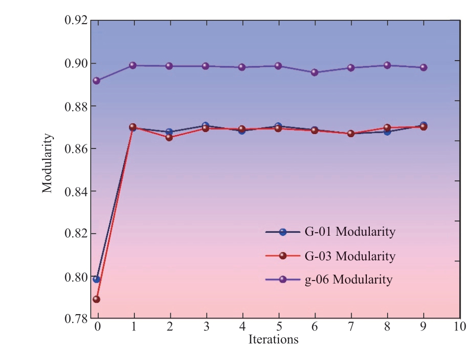
Fig.9 Modularity variation for different WTs
Fig.10 shows the distribution of communities obtained using the Louvain algorithm division of the G-01 wind turbine.
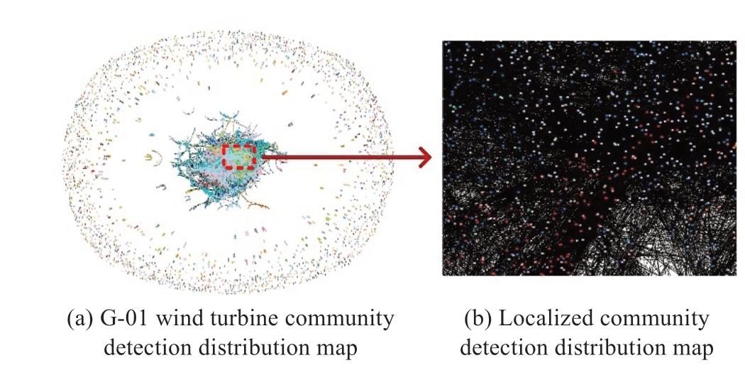
Fig.10 Diagram schematic of the community division for G-01 wind turbine
Fig.10 illustrates that under the Louvain algorithm, the detected communities are clearly divided into two parts:densely packed internal communities and scattered external communities, with each detected community represented by a different color.Densely packed internal communities indicate that these nodes exhibit similar patterns and are identified and clustered using the community detection algorithm.By contrast, the scattered external node communities represent potential outliers or patterns that differ from those in the main cluster.In the context of wind power generation, the densely packed communities represent wind speed and power data with similar attributes, whereas the scattered communities may correspond to special wind speed and power output relationships, such as high power output at low wind speeds or irregular data points caused by equipment failure.By removing these scattered communities,anomalous wind power data can be cleaned.
3.4 Horizontal community identification
To effectively remove Type II anomaly data from the WTs, each of the divided communities in Section 3.3 must be traversed to ascertain its height HSc and width WSc; when the community’s height-to-width ratio exceeds the threshold ε, the nodes inside the community must be removed.ε can be expressed as
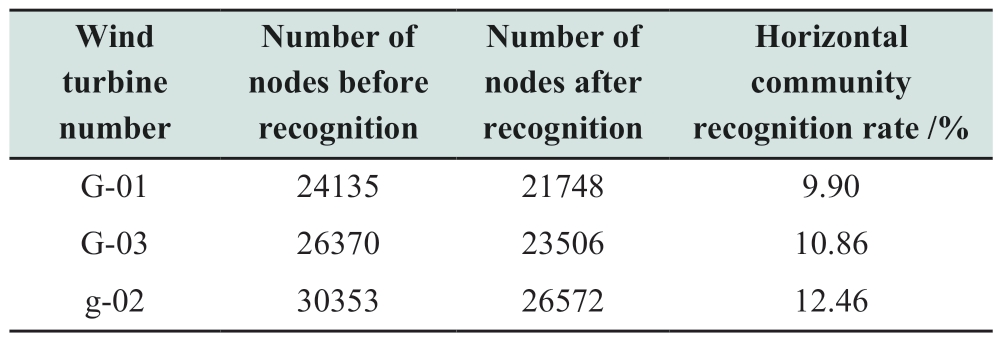
Taking WTs G-01, G-03, and g-02 as examples, the horizontal communities have been distinctly identified, as shown in Fig.11, and Table 2 indicates that the recognition rate ranges from 9.90% to 12.46%.
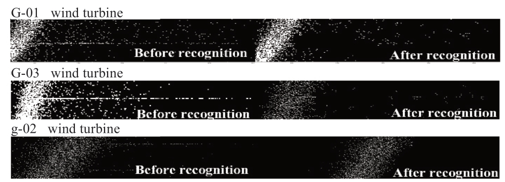
Fig.11 Recognition effects of horizontal communities for each wind turbine
Table 2 Recognition rate of horizontal communities for each wind turbine
3.5 Parameter optimization
After the community division, the undirected graph requires preliminary anomalous node cleaning.To validate the cleaning performance of the method, it is necessary to analyze the effect of different combinations of parameters of the inter-node boundary construction method, such as the capability of removing anomalous nodes in the undirected graph of the combination of the initial neighborhood radius r and connection attenuation coefficient s and the combination of community size (the community with how many number of nodes it contains) and node degree threshold.The analysis results for the G-01 turbine are presented in Fig.12.
The relationship among the size of the neighborhood radius r, the size of the communities removed, the node degree threshold setting, and the total number of nodes in the undirected graph is depicted in Fig.12(a).As the red folded line illustrates, an increase in the initial neighborhood radius r increases the likelihood that more edges will be established between more nodes, which helps the community detection algorithm retain more nodes.Furthermore, many anomalous feature nodes may be removed by eliminating small communities (purple folded line) and setting the size of the internode degree threshold (blue folded line).Figure 12 (b) shows that by simultaneously adjusting r and the connectivity decay coefficient s, the number of edges in the graph increases rapidly.The increase in the number of edges implies that the connectivity of the graph is enhanced for a given combination of parameters; thus, Fig.12 (c)eliminates a large number of anomalous nodes characterized by small communities and low node degrees by limiting the node degree threshold and the number of nodes in the communities.The combined consideration of r, s, and the parameter combination of community size and node degree threshold enhances the possibility of the algorithm cleaning more anomalous nodes.
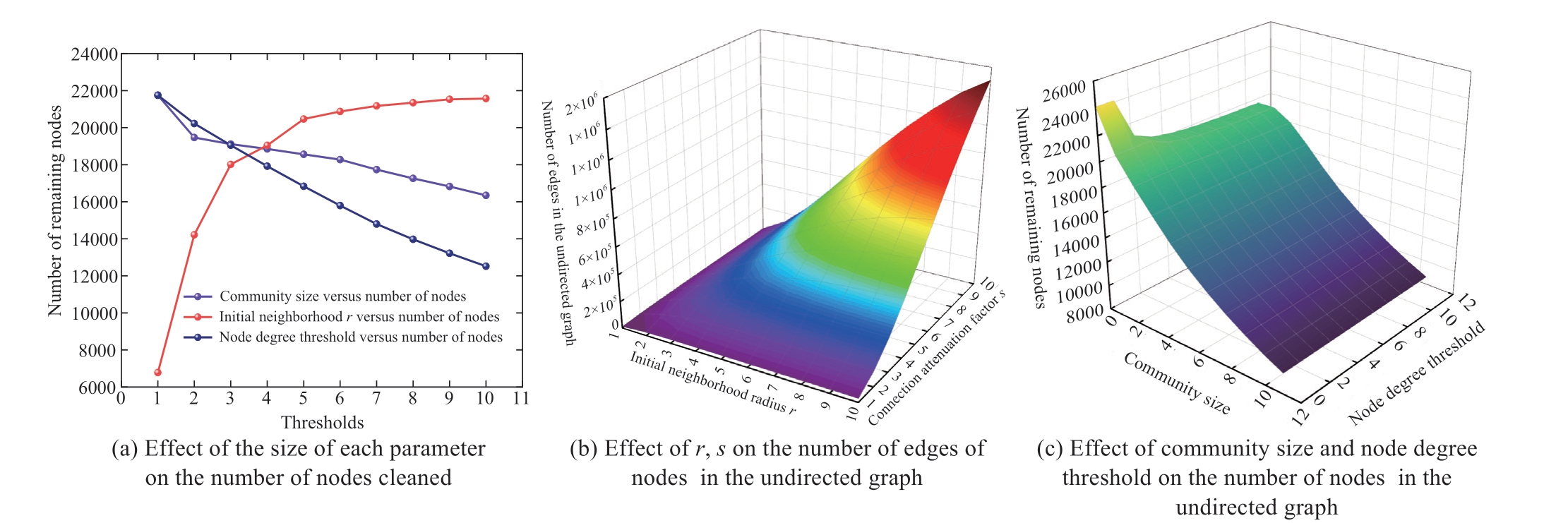
Fig.12 Effect of different parameter combinations on the number of nodes and edges in an undirected graph
3.6 Subject data extraction
Following the initial cleaning of the anomalous data in the second stage, additional representative subject data are extracted using the opening operation in mathematical morphology [20] to further remove noise and smooth the contour edges of the WPC image I.The MMO can be expressed as:

where E(I,S) is the erosion operation that removes the small noise at the edge of the image by applying the structure unit S of size n×n to the foreground pixels, and D(I,S) is the expansion operation that expands the pixels at the edge of the image using the structure unit S to smooth the image.The open operation I ◦S is a combination of image erosion and subsequent expansion to obtain a WPC image with low noise and smooth edges by adjusting the structuring unit S.The mathematical morphology operation is shown in Fig.13.
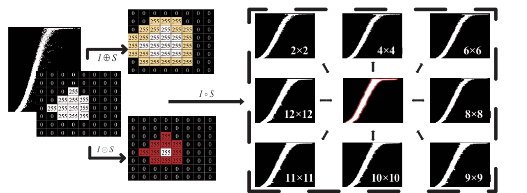
Fig.13 Mathematical morphological operations on WPC images after anomalous data cleaning
Finally, the final anomaly data cleaning is completed by mapping the determined WPC subject image back to the normal wind power points; the cleaning effect of the CWPAD-IPCDA method on the three types of anomalous data is shown in Fig.14.
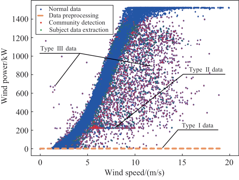
Fig.14 Effectiveness of the CWPAD-IPCDA method for cleaning three anomalous data patterns
4 Comparison of anomaly data cleaning methods
To evaluate the effectiveness of the proposed methodology for data cleaning, SCADA datasets from 25 WTs across two wind farms were processed using four distinct algorithms: the CWPAD-IPCDA method, improved isolated forest algorithm [21], DBSCAN algorithm [22],and image-based algorithm (IB) [16][20].The outcomes of these id="generateCatalog_13" style="text-align: left; text-indent: 0em; font-size: 1.2em; color: rgb(195, 101, 0); font-weight: bold; margin: 0.7em 0em;">4.1 Datasets and setup
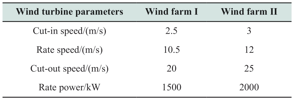
This study utilized original SCADA data from 25 WTs across two wind farms in Gansu Province, China, recorded every ten minutes from 2017/11/1 to 2019/12/31.The datasets for the two wind farms spanned 245 and 365 days,respectively.The specifications of the WTs are listed in Table 3.To quantitatively assess the cleaning performance of various algorithms, an expert was invited to analyze the wind turbine operation logs, with an understanding of each type of anomaly, and accurately label the original datasetswith normal and abnormal tags to clearly identify actual normal data and anomalies.All data cleaning algorithms were validated using Python version 3.8, operating on a laptop equipped with an AMD Ryzen 7 5800H CPU @ 3.20 GHz, an NVIDIA GeForce RTX 3060 GPU, and 16 GB of RAM.
Table 3 Specification of WTs for two wind farms
4.2 Performance evaluation
To comprehensively evaluate all the comparison algorithms, this study employed visualization of the wind power curves before and after cleaning, along with wind power curve modeling, to intuitively demonstrate the effectiveness of the cleaning process.Additionally, the identification accuracy (Precision, P), recall rate (Recall,R), and overall accuracy (F1—Score) were introduced to quantitatively assess algorithm performance.Finally, the data deletion rates and computation times for each algorithm were calculated and compared.
1) Power curve modeling
In references [5] and [23], methods for modeling wind power curves were proposed,which were applied to wind power data cleaned by various abnormal data identification algorithms.In addition, the sum of squares due to error(SSE), coefficient of determination (R²), and root mean square error (RMSE) were used to assess the goodness of fit(GoF) of the power curves, thereby validating the cleaning performance of the algorithms.
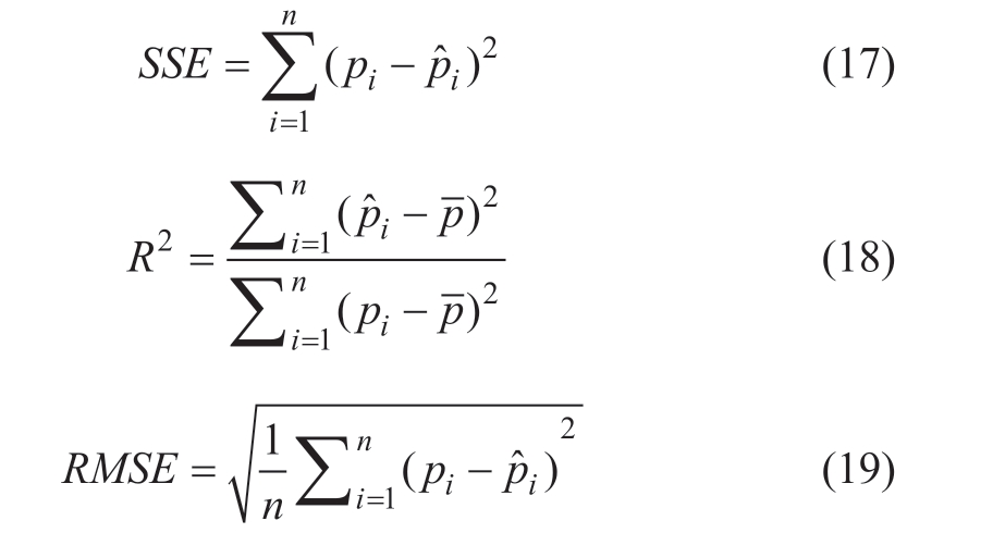
Where n is the number of observation points, pi is the ith actual observation, pˆi is the ith fitted value, and p is the average of all the actual observations.
This study employed a deep learning model that integrates attention mechanisms with a one-dimensional convolutional neural network to model the wind power curve.The model configuration included three hidden layers with dimensions of 128, 128, and 64.The ReLU activation function was used and the model was optimized using a gradient descent (Adam) algorithm with a learning rate of 0.001 over a maximum of 50 iterations.The analysis involved comparing GoF indicators across different datasets,both before and after applying the same algorithmic cleaning, and across the same dataset following different algorithmic cleanings.Lower SSE and RMSE values,coupled with higher R2 values, demonstrate a superior fit of the model to the actual data, thus more accurately reflecting the true characteristics of the wind turbine data and the effectiveness of the cleaning algorithm.
2) Metrics
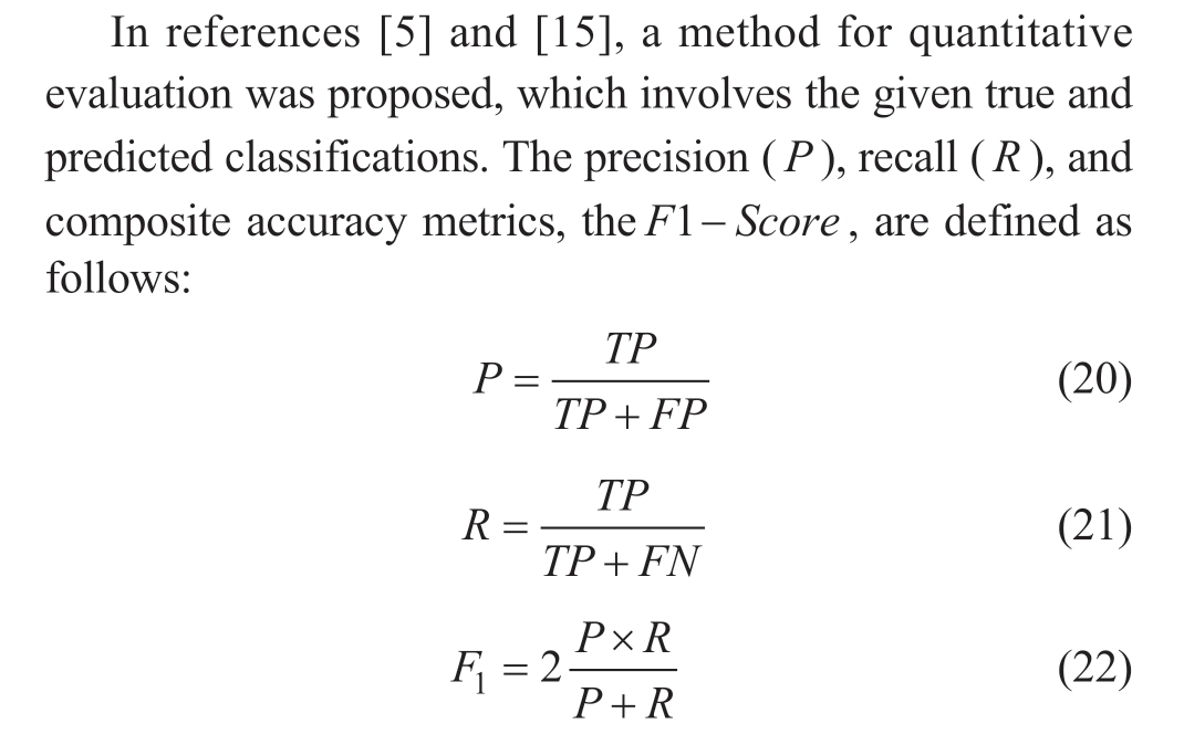
where TP is the number of data points that are correct values and correctly recognized as normal, FP is the number of data points that are outliers but incorrectly recognized as normal, and FN is the number of data points that are correct values but incorrectly recognized as outliers.Higher values of these metrics indicate better performance of the algorithm in data cleaning.
4.3 Algorithm parameterization
The improved isolated forest, DBSCAN, IB, and CWPAD-IPCDA algorithms were used to simulate and validate the dataset.
The DBSCAN algorithm uses density-based spatial clustering to cluster data by identifying regions with sufficiently high density.This algorithm relies on two essential parameters: eps (ε, neighborhood radius) and min-samples (minimum number of samples within the neighborhood).The eps parameter defines the neighborhood range of a point; if the distance between two points is less than eps, they are grouped into the same cluster.Meanwhile, the min-samples parameter specifies the minimum number of data points required to form a cluster;a point is considered a core point and can form a cluster if its neighborhood contains at least min-samples of data points.For outlier detection, DBSCAN labels the data points that cannot be assigned to any cluster as outliers.In this experiment, the DBSCAN algorithm was implemented using the scikit-learn library, and optimal performance was achieved when eps is set to 0.5 and min-samples to 5.
Isolation forest is a tree-based algorithm that calculates an anomaly score for each data point based on the path length in an isolation tree, with scores close to 1 indicating a higher likelihood of being an outlier.This study adapted the isolation forest construction method outlined in Ref.[21]and incorporated density clustering to enhance the detection of anomalies in wind turbine data.Initially, the isolation forest’s parameters, specifically n_estimators (number of trees), were fine-tuned using the scikit-learn library.The contamination parameter (the expected proportion of outliers) was set to ‘auto’, allowing the algorithm to estimate the proportion of outliers internally.Subsequently,clustering techniques were employed to further scrutinize the data points deemed normal by the isolation forest,particularly those misclassified as normal at the boundaries.The experimental results indicate that setting n_estimators to four yields the optimal data cleaning performance.
The algorithm based on image processing transforms wind power data into an image format, subsequently employing techniques such as contour detection and mathematical morphological operations to enhance the representation of data points within the image while simultaneously reducing background noise for intuitive anomaly detection.Following the methodologies outlined in References [16] and [20], this experiment utilized mathematical morphological operations and median filtering of binary images for anomaly data cleaning in wind power curves.Morphological operations, specifically the open and close operations, employ a 6×6 square kernel(morph_kernel = np. ones((6, 6)) with an iteration count of six (iterations=6).The purpose of multiple dilations is to enlarge the data point regions within the image, thereby facilitating the connection of adjacent pixels into continuous areas.Median filtering, through substituting each pixel’s value with the median of the neighboring pixel values,effectively eliminates isolated noise points with a kernel size of 3×3.The results demonstrate that the application of mathematical morphological operations and median filtering effectively removes anomalies from the wind power data.
4.4 Algorithms performance analysis
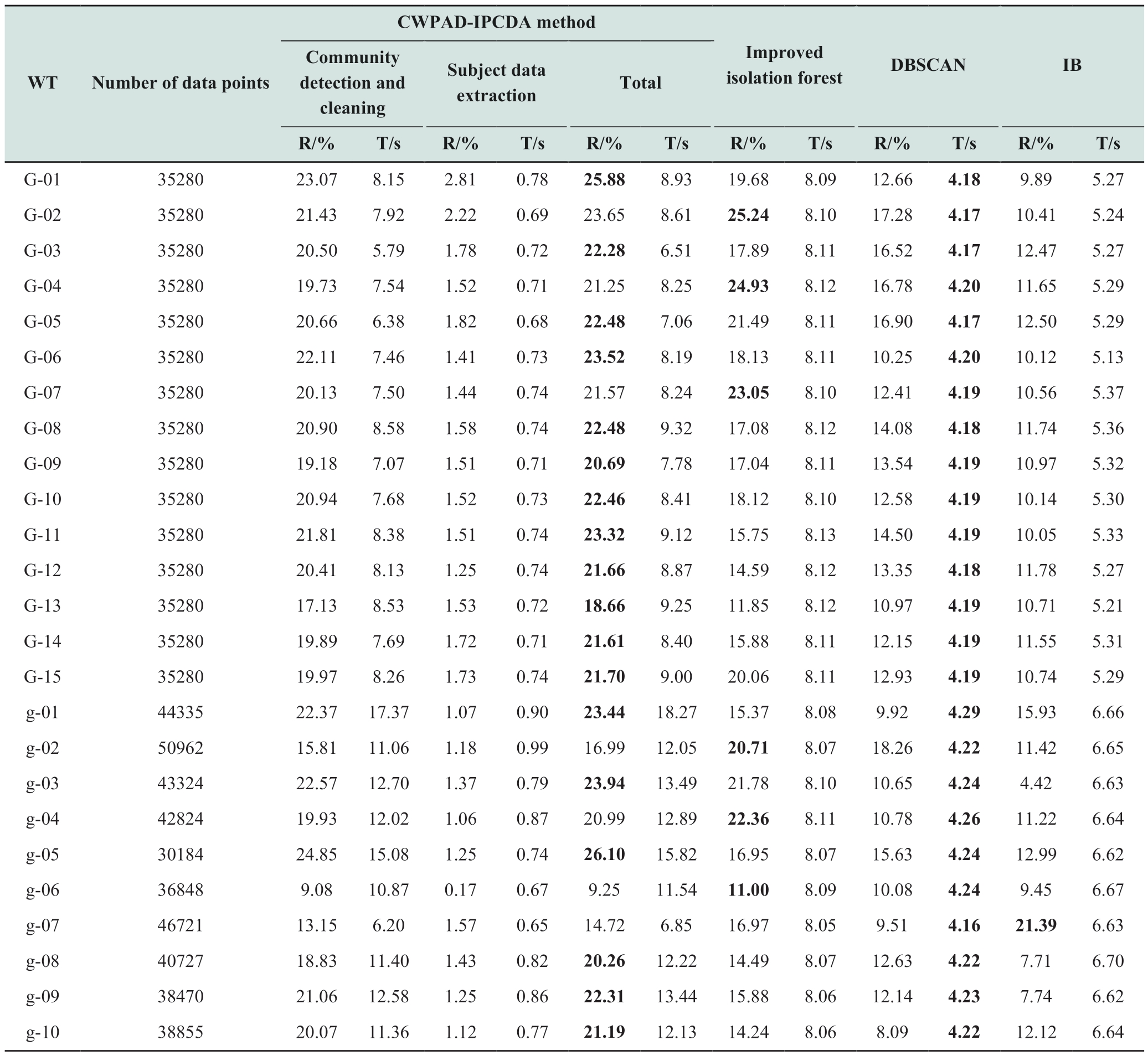
Table 4 presents the anomaly removal rates (R, %) and computation times (T, s) for various datasets in Wind Farms I and II, as processed by the four different algorithms.Higher removal rates indicate a greater ability to identify anomalies [5].The results show that the CWPAD-IPCDA method has the highest anomaly data cleaning performance,with an average cleaning rate of 21.29%, which is 3.27%,8.31%, and 10.11% higher than those of the improved isolation forest, DBSCAN, and IB algorithms, respectively.From Table 4, it is evident that DBSCAN required the shortest cleaning time.This is attributed to its utilization of a spatial indexing structure (R-tree) to expedite theneighborhood search process, thereby enhancing its efficiency in locating style="vertical-align: middle; text-align: center;">
Table 4 Wind farm Ⅰ and II anomaly data cleaning results
From Tables 5 and 6, it is evident that the CWPADIPCDA method demonstrated R2 values closer to 1 and lower RMSE values than the other three algorithms for both the cleaned models and models subjected to different cleaning algorithms on the same dataset.This suggests that the CWPAD-IPCDA method is more efficient in mitigating the interference caused by abnormal data, thereby enhancing the robustness of the models.Moreover, Table 6 reveals that the DBSCAN algorithm exhibited better performance across all three metrics compared to the improved isolation forest and IB algorithms.Despite its lower removal rate,the DBSCAN algorithm effectively eliminated significant outliers while maintaining a lower false detection rate.By contrast, despite having higher removal rates, the improved isolation forest and IB algorithms were susceptible to misidentification.
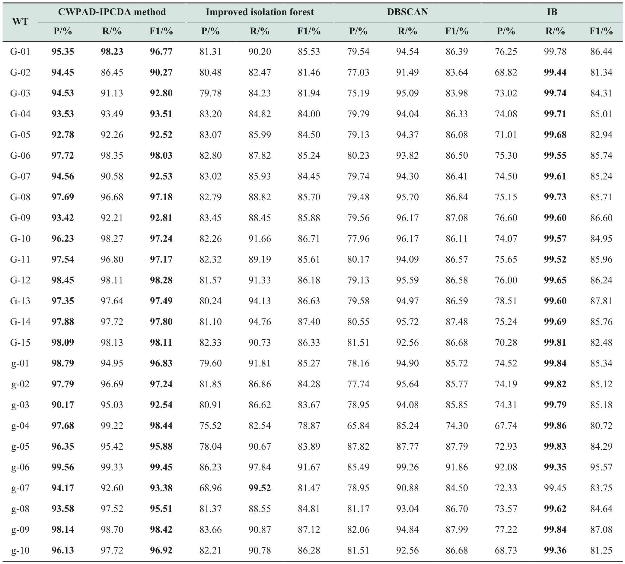
The identification and cleaning of anomalous wind speed-power data inevitably resulted in the accidental deletion of some normal data to compromise the integrity of normal data [8].Table 7 shows that the proposed method significantly surpassed the improved isolated forest and the DBSCAN algorithms in terms of accuracy P, identification rate R, and F 1- Score.However, compared with the CWPAD-IPCDA method, the IB algorithm exhibiteda higher R.This is attributed to the IB algorithm’s effective use of MMO operations and median filtering to connect adjacent pixels in images into larger continuous areas, which also results in a very high TP and very low FN.However,the use of MMO operations and median filtering also leads to an increase in FP, thereby reducing its accuracy P.In contrast, the method presented in this paper achieved higher accuracy in P and F Score 1- , exhibited a lower rate of erroneous data cleaning, and demonstrated superior comprehensive performance.
In Fig.15, green and blue points represent the original data and normal data points, respectively, while the redcurves represent the fitted power curves for the datasets before and after cleaning.In Figs.16-19, red and blue points represent the data identified as normal and abnormal,respectively, by each algorithm.From Figs.15 to 19, it can be observed that the CWPAD-IPCDA method effectively identified the power limitation points caused by grid curtailment for these six WTs.Meanwhile, the fitted wind power curves are the smoothest and have the best GoF.
Table 5 Modeling statistics before and after cleaning
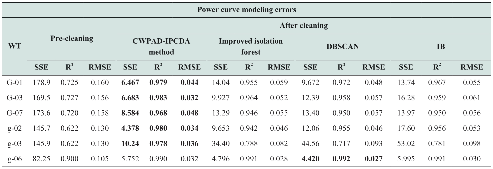
Table 6 Power curve modeling statistics
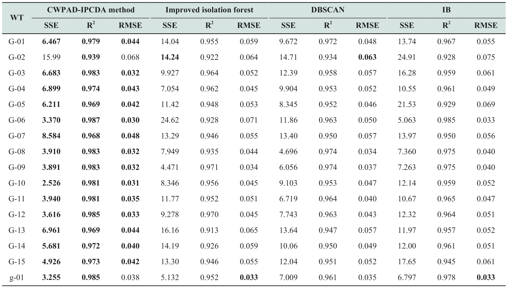
continue

Table 7 Metrics of data cleaning results for all datasets by four methods
Compared with the other three algorithms, the proposed algorithm comprehensively removes Type II and Type III anomalies within the WTs.Comparisons from Figs.15 to 19 reveal that the DBSCAN algorithm, due to its reliance on the ε and min-samples parameter choices, the DBSCAN algorithm cannot easily identify the stack anomalies horizontally that are very close to each other in feature space (e.g., WTs G-03 and g-03).This makes parameter selection challenging and ineffective for anomaly detection to lead an increase in false positives (FP), thereby reducing the accuracy P and the accuracy of modeling.Conversely,compared with DBSCAN and IB algorithms, the improved isolation forest algorithm, particularly in areas where normal and anomalous data overlap significantly at the curve's peak (e.g., WTs G-07 and g-03), employs more aggressive and sensitive tree division and density clustering methods to avoid misclassifying anomalies as normal to result in a lower number of FP and higher accuracy P.However, this approach also leads to a substantial deletion of normal data,which leads to the number of true positives (TP) reduced and false negatives (FN) increased, thereby lowering the recall (R) and the accuracy of modeling.When dealing with poor-quality datasets, such as those from WTs G-03 and g-03,the IB algorithm's sole reliance on mathematical operations within the image may fail to comprehensively consider the complex structures and features present in the data.This limitation prevents the algorithm from fully leveraging the potential information within the data, thereby restricting the accuracy and robustness of the cleaning methods.
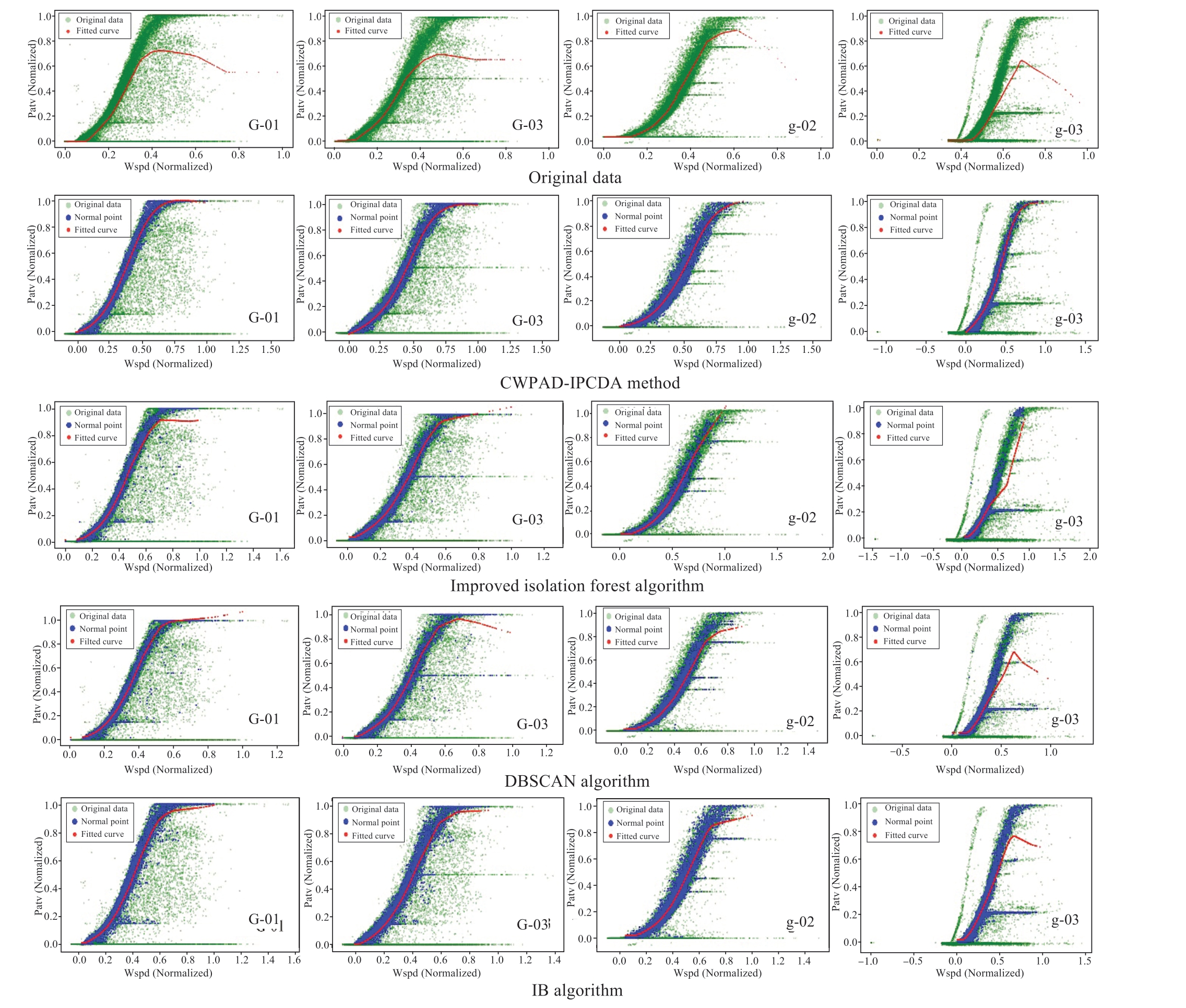
Fig.15 Wind power curve modeling
Combining Tables 4-7 and Figs.15-19, we can draw the following conclusions.Compared with the other three algorithms, the CWPAD-IPCDA method employs the Louvain algorithm in the community aggregation stage,enabling the observation of the data distribution and structure within each community at different granularities.It detects horizontally stacked regions, which constitute about 10-12% of the total dataset.By restricting node degree thresholds and community node sizes, it achieves an average a preliminary average cleaning rate of 18.77-20.52% for wind farms I and Ⅱ, efficiently removing Type II and Type III anomalies.Thus, a low number of (FP) and (FN) in the data are guaranteed.In addition, incorporating mathematical morphological operations allows for further smoothing of the WPC image edges, and noise refinement yields more representative data, resulting in a high number of (TP) data recognition and ensures high recognition accuracy P and recall R.After data cleaning, the SSE error in the wind power curve modeling was reduced by 6.887 compared with the mean SSE of the other three algorithms, while R2 was improved by 0.035 and the RMSE was reduced by 0.011.The method proposed in this study demonstrates the highest data identification accuracy, with an average overall F 1- Score that surpasses those of the other algorithms discussed by approximately 10.49%.Its performance in recognizing and cleaning anomalous data was significantly superior to that of the three aforementioned algorithms.
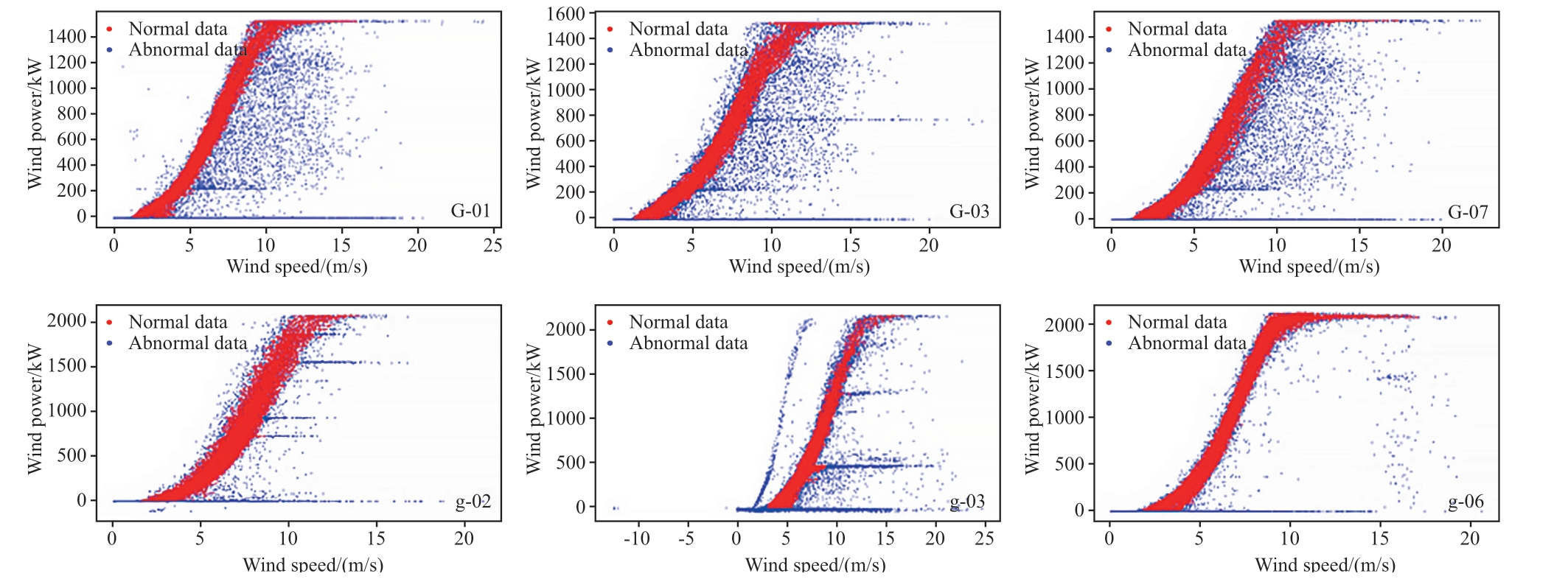
Fig.16 CWPAD-IPCDA method
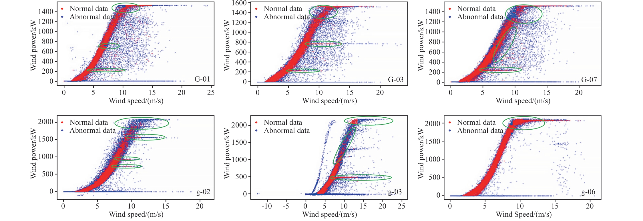
Fig.17 Improved isolated forest algorithm
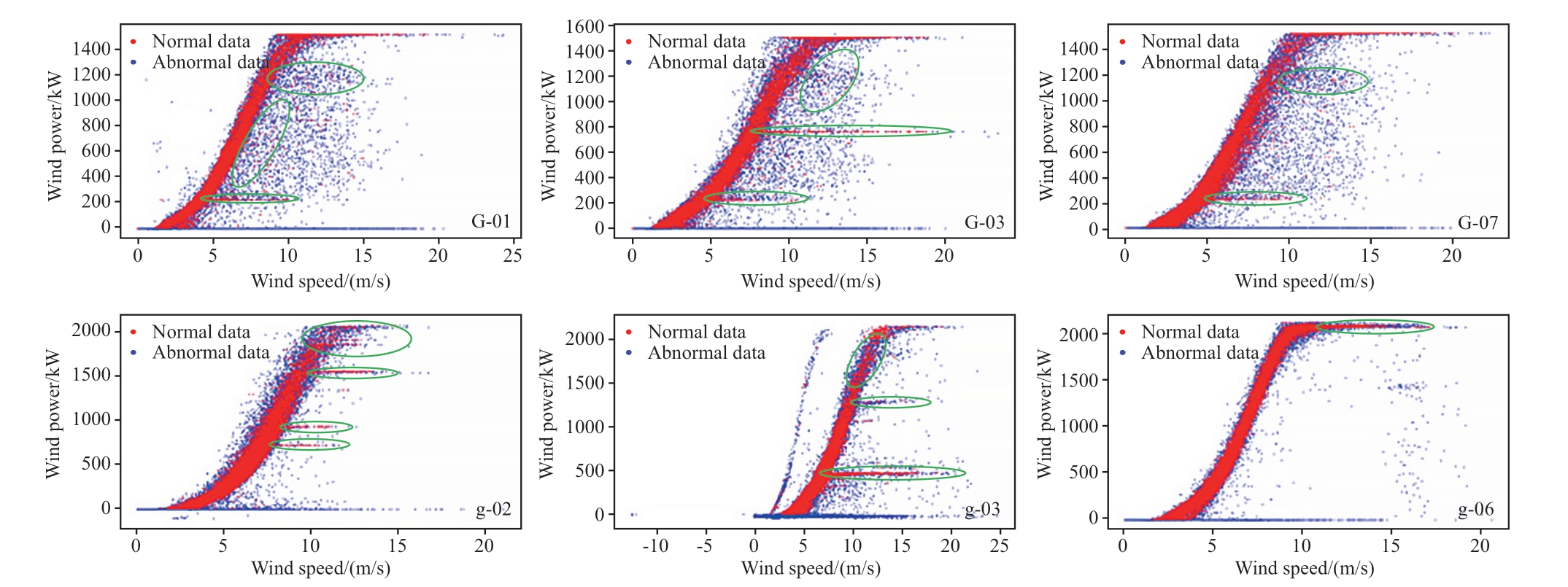
Fig.18 DBSCAN algorithm
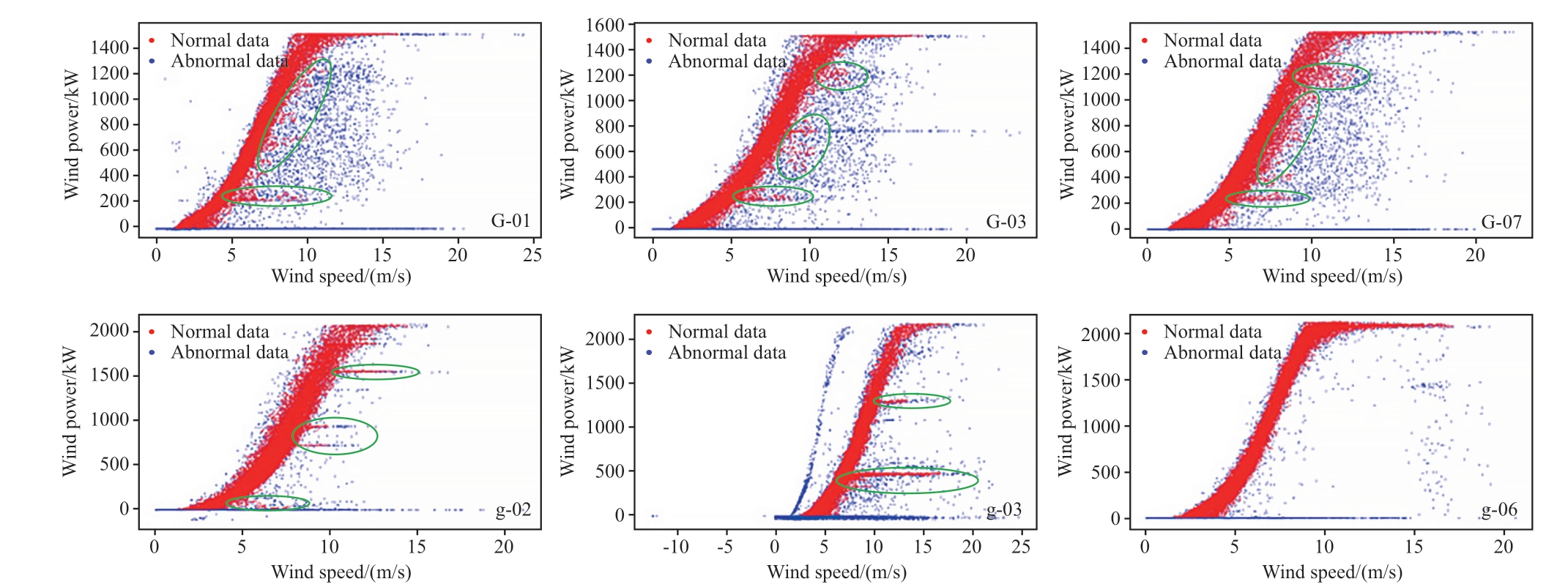
Fig.19 IB algorithm
5 Conclusion
Through theoretical derivation, simulation validation,and arithmetic example analysis of a method for cleaning wind power anomaly data by combining image processing with community detection algorithms (CWPAD-IPCDA)proposed in this study, the following conclusions can be drawn: (1) Compared to the other three algorithms,the Louvain community detection algorithm can quickly delineate obvious community structures after 2-4 rounds of modularity optimization, in which the horizontal community recognition rate accounts for approximately 10-12% of the total data.(2) Combining the graph-theoretic approaches and the delineated communities, about 18.77-20.52% of the anomalous nodes in the undirected graph can be eliminated by restricting the node degrees and the community structures under the combined parameters, which efficiently removes the Type Ⅱ and Type Ⅲ anomalous nodes while highlighting the more representative community features.(3)The use of open operations in image processing techniques not only further refines the WPC edge noise while preserving the subject data but also improves the overall cleaning performance of the CWPAD-IPCDA method by approximately 0.17-2.81%.(4) The experimental results demonstrate that the CWPAD-IPCDA method surpasses the other three algorithms, achieving an average data cleaning rate that is approximately 7.23% higher.The mean SSE of the dataset after cleaning was approximately 6.887 lower than that of the other algorithms.Moreover, the mean of overall accuracy, as measured by the F1-score, exceeded that of the others by approximately 10.49%, indicating its superior performance in the identification and cleaning of wind power anomaly data.
In summary, the CWPAD-IPCDA method proposed in this study provides a new solution and a theoretical basis for wind power anomaly data cleaning and wind power prediction accuracy improvement.
Acknowledgments
This work was supported by the National Natural Science Foundation of China (Project No.51767018) and Natural Science Foundation of Gansu Province (Project No.23JRRA836).
Declaration of Competing Interest
We declare that we have no conflict of interest.
Reference
[1]Yao G, Yang H M, Zhou L D, et al.(2021) Development status and key technologies of large-capacity offshore wind turbines.Automation of Electric Power Systems, 45(21): 15
[2]Chinese Wind Energy Association (2022) Statistical Briefing on Wind Power Lifting Capacity in China, Wind Energy, 2023(04):40-56 (in Chinese)
[3]Wu Y B, Zhang J Z, Yuan Z X, et al.(2023) Review on identification and cleaning of abnormal wind power data for wind farms.Power System Technology, 47(06): 2367-2380 (in Chinese)
[4]Yang J X (2022) Research on wind power forecasting method considering the characteristics of wind data.Central South University
[5]Luo Z H, Fang C Y, Liu C L, et al.(2022) Method for cleaning abnormal data of wind turbine power curve based on density clustering and boundary extraction.IEEE Transactions on Sustainable Energy.13(2): 1147-1159
[6]Li X Y (2023) Abnormal data processing method of wind turbine power curve based on combinatorial algorithm.Distributed Energy, 8(03): 73-78 (in Chinese)
[7]Kusiak A, Verma A (2013) Monitoring wind farms with performance curves.IEEE Transactions on Sustainable Energy,4(1): 192-199
[8]Zou T H, Gao Y P, Yi H J, et al.(2022) Processing of wind power abnormal data based on Thompson tau-quartile and multipoint interpolation.Automation of Electric Power Systems,44(15): 156-162 (in Chinese)
[9]Bilendo F, Meyer A, Badihi H, et al.(2022) Applications and modeling techniques of wind turbine power curve for wind farms—a review.Energies, 16(1): 180
[10]Park J Y, Lee J S, Oh K Y, et al.(2014) Development of a novel power curve monitoring method for wind turbines and its field tests.IEEE Transactions on Energy Conversion, 29(2014): 119-128
[11]Bilendo F, Badihi H, Lu N Y, et al.(2022) A normal behavior model based on power curve and stacked regressions for condition monitoring of wind turbines.IEEE Transactions on Instrumentation and Measurement, 71: 3520013
[12]Hu Y, Qiao Y L, Liu J Z, et al.(2019) Adaptive confidence boundary modeling of wind turbine power curve using SCADA data and its application.IEEE Transactions on Sustainable Energy, 10(3): 1330-1341
[13]Sun Z X, Sun H X (2019) Stacked denoising autoencoder with density-grid based clustering method for detecting outlier of wind turbine components.IEEE Access, 7: 13078-13091
[14]Wu Y B, Zhang J Z, Din Z U, et al.(2022) Anomaly data identification for wind farms based on composite machine learning.Journal of Renewable and Sustainable Energy, 14(6)
[15]Liang G Y, Su Y H, Chen F, et al.(2021) Wind power curve data cleaning by image thresholding based on class uncertainty and shape dissimilarity.IEEE Transactions on Sustainable Energy,12(2): 1383-1393
[16]Liu Y L, Zhang Y J, Wang L, et al.(2023) Wind farm abnormal operation data cleaning method based on piecewise image recognition, Renewable Energy Resources, 41(04): 500-506 (in Chinese)
[17]Mei Y, Li X, Hu Z C, et al.(2021) Identification and cleaning of wind power data methods based on control principle of wind turbine generator system.Journal of Chinese Society Engineering,41(04): 316-322+329 (in Chinese)
[18]Blondel V D, Guillaume J L, Lambiotte R, et al.(2008) Fast unfolding of communities in large networks.Journal of Statistical Mechanics: Theory and Experiment, 2008(10): P10008
[19]Newman M E J (2004) Analysis of weighted networks.Physical Review E, 70(5): 056131
[20]Long H, Sang L W, Wu Z J, et al.(2020) Image-based abnormal data detection and cleaning algorithm via wind power curve.IEEE Transactions on Sustainable Energy, 11(2): 938-946
[21]Feng W Z, Zhu S P, Zhao Z H (2021) Comparative study on detection methods of wind power abnormal data.Advanced Technology of Electrical Engineering and Energy, 40(07):55-61(in Chinese)
[22]Yan J, Zhang H, Liu Y, et al.(2019) Uncertainty estimation for wind energy conversion by probabilistic wind turbine power curve modelling.Applied Energy 239: 1356-1370
[23]Yesilbudak M (2018) Implementation of novel hybrid approaches for power curve modeling of wind turbines.Energy Conversion and Management, 171: 156-169

Scan for more details
Received: 26 February 2024/Revised: 28 March 2024/Accepted: 6 May 2024/Published: 25 June 2024
Qiaoling Yang
winds-qiaoer@163.com
Kai Chen
JaMeZz9176@163.com
Jianzhang Man
manjz1122@163.com
Jiaheng Duan
15829024090@163.com
Zuoqi Jin
13659359837@163.com
2096-5117/© 2024 Global Energy Interconnection Group Co.Ltd.Production and hosting by Elsevier B.V.on behalf of KeAi Communications Co., Ltd.This is an open access article under the CC BY-NC-ND license (http: //creativecommons.org/licenses/by-nc-nd/4.0/ ).
Biographies

Qiaoling Yang received PhD in renewable energy power generation and smart Grid from Lanzhou University of Technology in 2020.She is working at Lanzhou University of Technology.Her research interests include power electronics and power transmission,renewable energy generation and smart grids,and motor design and control.

Kai Chen is currently pursuing the master’s degree in electrical engineering at Lanzhou University of Technology.He mainly researches new energy prediction and artificial intelligence and their applications in power systems at present.

Jianzhang Man is currently pursuing the master’s degree in electrical engineering at Lanzhou University of Technology.He mainly researches distributed generation,virtual synchronous generator technology, and their applications in power systems.

Jiaheng Duan is currently pursuing the master’s degree in electrical engineering at Lanzhou University of Technology.He mainly researches new energy power system inertia prediction in power systems.

Zuoqi Jin is currently pursuing the master’s degree in electrical engineering at Lanzhou University of Technology.He mainly researches distributed generation, virtual synchronous generator technology, and their applications in power systems.
(Editor Yanbo Wang)
