0 Introduction

In 2020,China put forward the goal of “carbon peak and carbon neutrality,” which proposed the development direction of new energy as the main body of the power system [1-4].In the low-carbon situation,the proportion of new energy is rising rapidly,and there are many interactive devices that can be accessed,such as electric vehicles and distributed power sources.Power systems have greatly increased the difficulty in maintaining a balance between power and electricity in the case of a high proportion of renewable energy and a high proportion of power electronic equipment.To accurately grasp the form of power supply and demand and ensure power supply,power-load forecasting is particularly important.

With the increase in the complexity of power systems,a generalized load exists for the new energy power system[5-7].The generalized load is the sum of renewable energy output,flexible resources,and actual electricity demand on the load side in the context of a high proportion of renewable energy integration and the continuous development of smart grids.A generalized load has the main characteristics of load component diversification,diversified influencing factors,complex spatiotemporal characteristics,and strong uncertainty,which cause significant difficulties in load forecasting.The main difficulty is that the changing trend is not obvious and is difficult to predict.Time series do not have clear rules,and it is difficult to use traditional methods.Many factors influence the generalized load,and it is difficult to determine the correlation between them.

The traditional load forecasting method primarily studies the temporal characteristics of the load,uses neural networks,machine learning,and other methods to construct the load forecasting model,and has achieved fruitful research results.Reference [8] used the EEMDGRU-MLR (EGM) method,combining ensemble empirical mode decomposition (EEMD),a gate recurrent unit neural network (GRU),and multiple linear regression (MLR) for load forecasting.However,because of its large number of parameters,complex structure,and lack of better use of shallow features,gradient disappearance can easily occur.Therefore,problems remain in practical applications.Reference [9] used a model containing convolutional layers and bidirectional propagating LSTM and GRU recurrent layers to predict the load of the next hour and achieved good prediction results.However,the influencing factors considered are single and the common influence of multiple factors is not considered.The above-mentioned load prediction method uses the time-series curve as the input of the prediction model;the information contained in the load curve cannot be deeply explored,and the adaptive and selflearning abilities of the model need to be improved.

Recently,Deep Learning has developed rapidly,and its performance in the field of image processing has become particularly prominent.Successful cases of data image analysis have been reported.In [10],the theoretical basis and technical systems of deep learning have been summarized.Based on the actual demand of the power system,the key application areas and values of deep learning in power system data processing are summarized based on image and spatiotemporal data.In [11],the 96-point load data are converted into a 10×10 grayscale matrix,and a generative adversarial network was used for training,which realized the reconstruction of missing power data in the distribution network.However,when the data to be reconstructed differ from the current training data,the reconstruction effect could deteriorate.In [12],commercial load data were converted into color images and trained using a convolutional neural network (CNN)model,and cluster analysis was performed.However,because of the three-dimensional color images generated,the training speed of the model was significantly reduced.In[13],the discrete results of the slope soil random field were transformed into digital images to improve the stability of the calculation results.However,studies on highly efficient image-generation methods are lacking.

To address the above problems,this study proposes a novel generalized graphical load forecasting method based on modal decomposition.The DBSCAN clustering algorithm is used to establish generalized load scenarios under different wind and photovoltaic permeability [14,15].The generalized load images are trained by drawing on the superiority of DenseNet in image processing.Finally,the accuracies of the generalized load image prediction method and traditional prediction method are compared to verify the feasibility of graphical load data prediction.

The main contributions of this paper are summarized as follows.

1) Historical load,meteorological information,and day type were collected;the dataset was preprocessed using XGBoost,GBDT,and RF algorithms;and the feature contributions of various data are analyzed.

2) The generalized load data are decomposed into three sets of modes by modal decomposition,the RGB images are generated as the pixel values of the R,G,and B channels,and the image is diversified.

3) The processed images are trained and tested using the optimized DenseNet.

4) The base load,wind,and photovoltaic power data are selected,and the characteristic curves of the generalized load scenarios under wind and photovoltaic power generation with different permeabilities are obtained using the DBSCAN clustering algorithm.

5) According to the proposed graphical forecasting method,the feasibility of the generalized load graphical forecasting method is verified by comparing it with the traditional time-series forecasting method.

The remainder of this paper is organized as follows:Section 1 establishes the overall framework of the generalized load-forecasting method and analyzes its basic steps.In Section 2,a generalized load prediction model based on modal decomposition is established,including specific methods ranging from data processing to neural network optimization.Specifically,an innovative method for generating RGB images after modal decomposition is described in this paper.In Section 3,the generated RGB images are diversified to improve the generalization ability of the model.In Section 4,generalized load scenarios under different wind and photovoltaic permeabilities are established,and the generalized loads under different scenarios are predicted.Finally,we present our conclusions in Section 5.

1 Graphical generalized load forecasting framework

Generalized loads are primarily composed of distributed wind and photovoltaic generation,active loads,electric vehicles,and traditional distribution network loads.Wind and photovoltaic generation are mainly affected by climatic factors,such as wind size and light intensity.Market factors and demand-side responses primarily influence the active load.Electric vehicles are affected primarily by travel patterns and electricity prices.The load of a traditional distribution network is most affected by the weather and type of day.The generalized load is affected by a variety of factors,and there exists a coupling relationship between multiple load components,which makes research on load forecasting very difficult.This study primarily focuses on generalized loads under massive access to new energy sources,such as wind and photovoltaic generation.It is verified that the graphical prediction method has a high accuracy in different generalized load scenarios.The framework of the Generalized load graphical forecasting method is shown in Fig.1.

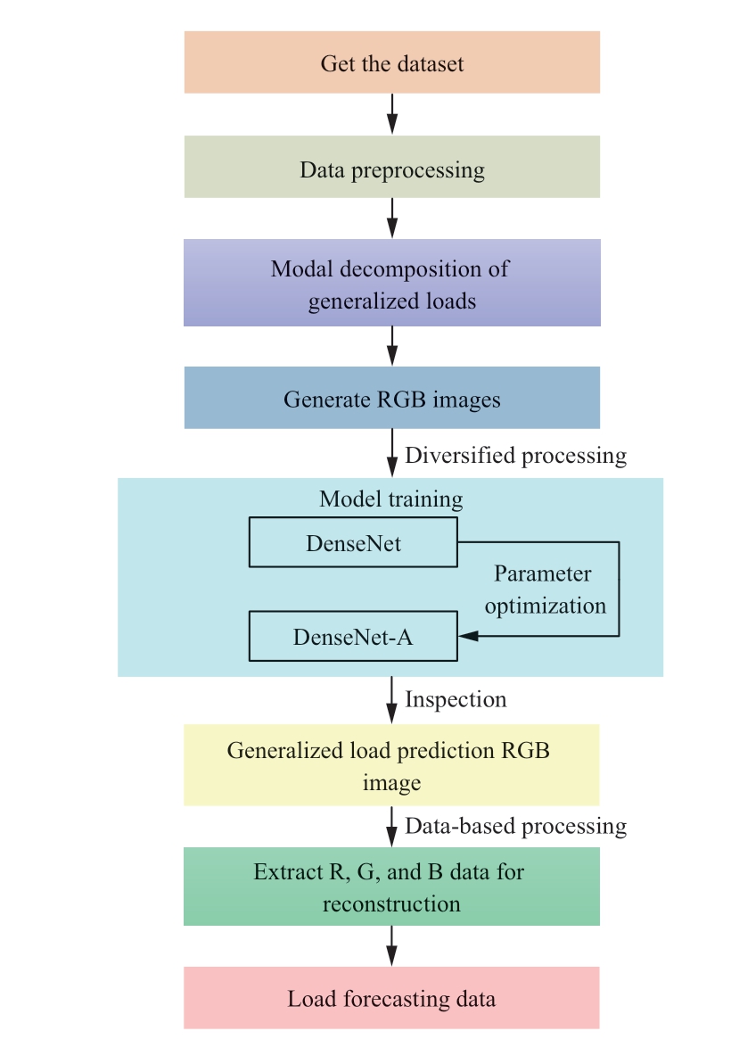
Fig.1 Generalized load graphical forecasting method framework

In Fig.1,the obtained dataset is preprocessed to fill the gaps in the historical load data.Various algorithms are used to reduce the dimensionality of the influencing factors,and factors with higher feature contributions are selected as the actual influencing factors.It is normalized and used as an input for the predictive model.The modal decomposition of the historical load data is performed,and the RGB image is obtained using the decomposition result.To improve the accuracy of image prediction,image is diversified.The processed image and influencing factor conditions are used as the input of the prediction model for training.DenseNet-A completes the testing and outputs the prediction image.Finally,the R,G,and B channel data of the prediction image were extracted to complete the reconstruction and obtain the generalized load prediction results.

2 Generalized load forecasting model based on modal decomposition

2.1 Date processing

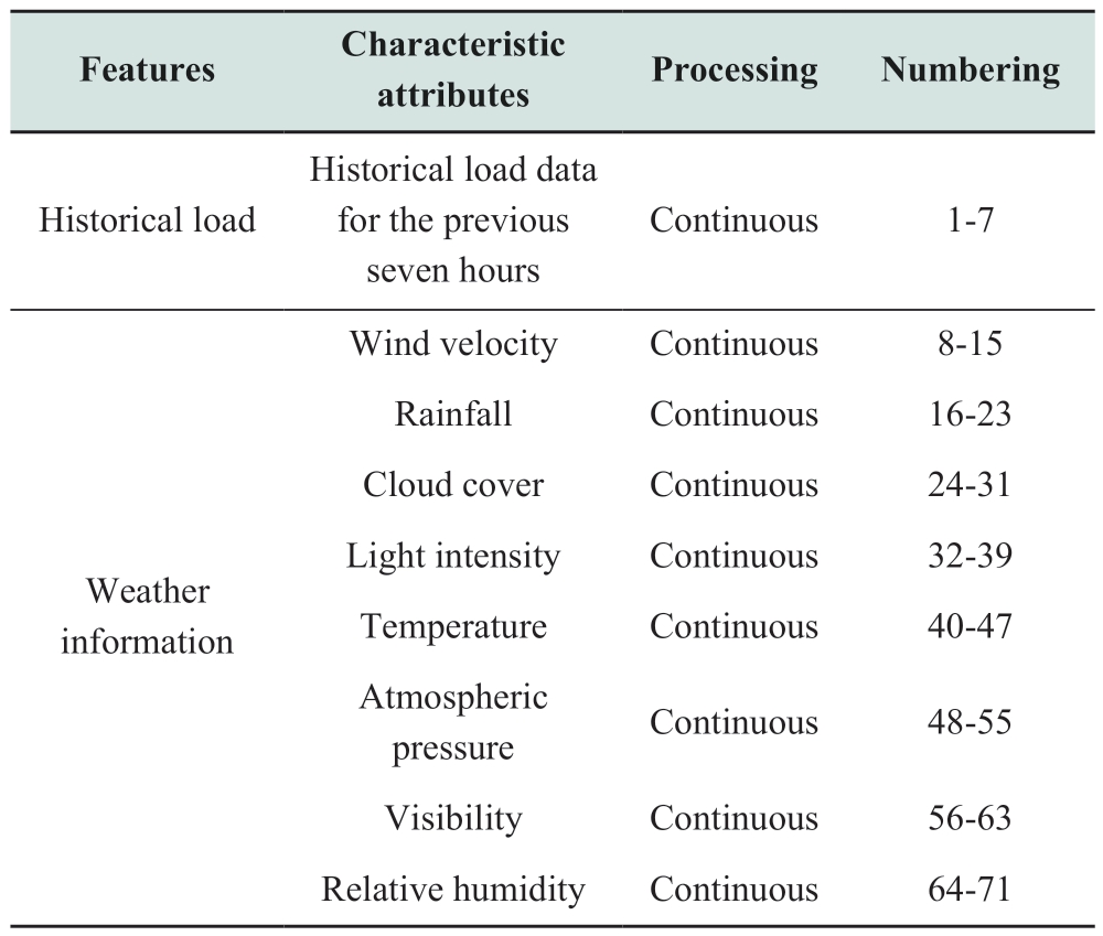
First,the linear interpolation method is used to complete and replace them [16,17].As there are too many influencing factors of the input,the uncertainty of the prediction results of the model increases;therefore,it is necessary to reduce the dimensionality of the data through feature contribution analysis.Calendar rules and meteorological factors were selected as input data in an artificial empirical manner.Meteorological factors include wind speed,rainfall,cloud cover,light intensity,temperature,air pressure,visibility,and relative humidity.Calendar rules include days of the week,months,and holidays.The attributes,processing methods,and number of selected input data points are listed in Table 1.

Table 1 Form and serial number of input attribute

continue

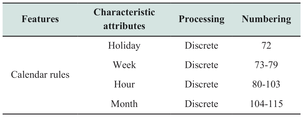
To avoid mutual interference between continuous data,one-hot data were used to discretize the characteristics of the week and month.Subsequently,the XGBoost,GBDT,and RF algorithms were used to obtain the feature contribution degree of the input information,and the results with similar feature contribution degrees were selected as the final influencing factor input information.The feature contributions calculated using the three algorithms are shown in Fig.2.

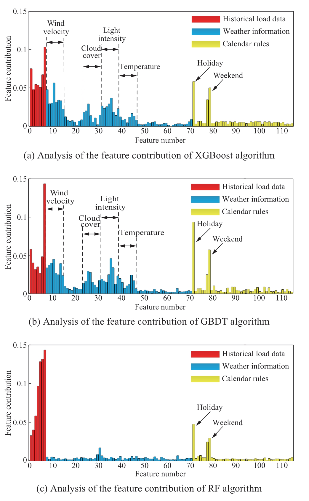
Fig.2 Feature contribution research based on different algorithms

As shown in Fig.2,the wind speed,light intensity,temperature,cloud cover,and other meteorological data have significant impacts on the load.Simultaneously,holidays and weekends also showed a high degree of characteristic contributions.Considering that features such as the week,hour,and month are discretely processed,although the feature contributions are sparser and more scattered,they are helpful for model training.Through further analysis in Fig.2,it can be observed that the XGBoost and GBDT algorithms yield similar results in the feature contribution analysis,and both can fully mine the internal features of the data;therefore,XGBoost (or GBDT) was selected for feature contribution analysis during training.

Finally,owing to the meteorological factors and calendar rules that affect the generalized load forecast,differences exist in the values of the symbols and orders of magnitude.Therefore,it is necessary to adjust the numerical range to be consistent via normalization.

2.2 Modal decomposition and visualization of load data

To make better use of the DenseNet network and make more use of the change information of various generalized loads in different permeability scenarios of wind and photovoltaic generation,the generalized loads were converted into RGB images by modal decomposition.For any integer I∈[0,224-1],the RGB color pixels can be based on (1),(2),and (3) to obtain pixel values.

The modal decomposition method adopts complete ensemble empirical mode decomposition with adaptive noise (CEEMDAN) [18].It can decompose raw load data into intrinsic mode functions (IMFs) containing different frequency ranges,and each IMF contains information regarding the original data in different frequency ranges.Therefore,the CEEMDAN decomposition of the original load time series is performed to obtain several IMFs that can realize the separation of different characteristics of the data.The feature information of different IMFs can then be converted into RGB images,which can deeply mine the rules contained in the data and effectively improve the prediction accuracy.

The CEEMDAN decomposition process is illustrated in Fig.3,where k in IMFk represents the number of iterations,and i in IMFki represents the i-th component after decomposition.

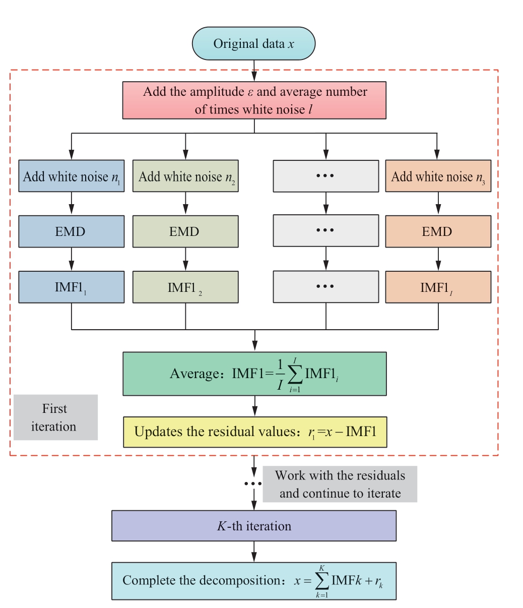
Fig.3 Decomposition process of complete ensemble empirical mode decomposition with adaptive noise

CEEMDAN improves the algorithm flow through EMD,combined with EEMD with low modal aliasing,and adds white noise.CEEMDAN combines the advantages of both worlds,such that the reconstruction error is almost zero and the speed of modal decomposition is improved.

Since each data point is of a different type,it must be normalized.The specific steps for visualization are as follows:

Step 1: Preprocess the raw load data to ensure that all serial data are time-sorted and maintained in the correct position.If data are missing in some locations,missing data or zeros can be removed or imputed from the dataset before analysis.

Step 2: CEEMDAN is used to process the raw load time series containing a large number of high-frequency and complex-frequency components.Following the frequency separation,several IMFs containing different frequency components are obtained.

Step 3: The number of modal decompositions is set to three,corresponding to the three channels of the RGB image,and the values are mapped to [0,1].It is then multiplied by 255 and rounded to obtain the pixel value of the three channels of the RGB image to obtain the RGB image containing multi-dimensional load data information.

Step 4: Extract the load data of the three channels in the RGB image of the predicted result and use the CEEMDAN to reconstruct it to obtain the load prediction result.

Fig.4 shows an inverse schematic diagram of the load data for 4 h and an RGB image with a sampling time interval of 15 min and an image size of 1 × 16 × 3 (rows ×columns × channels).

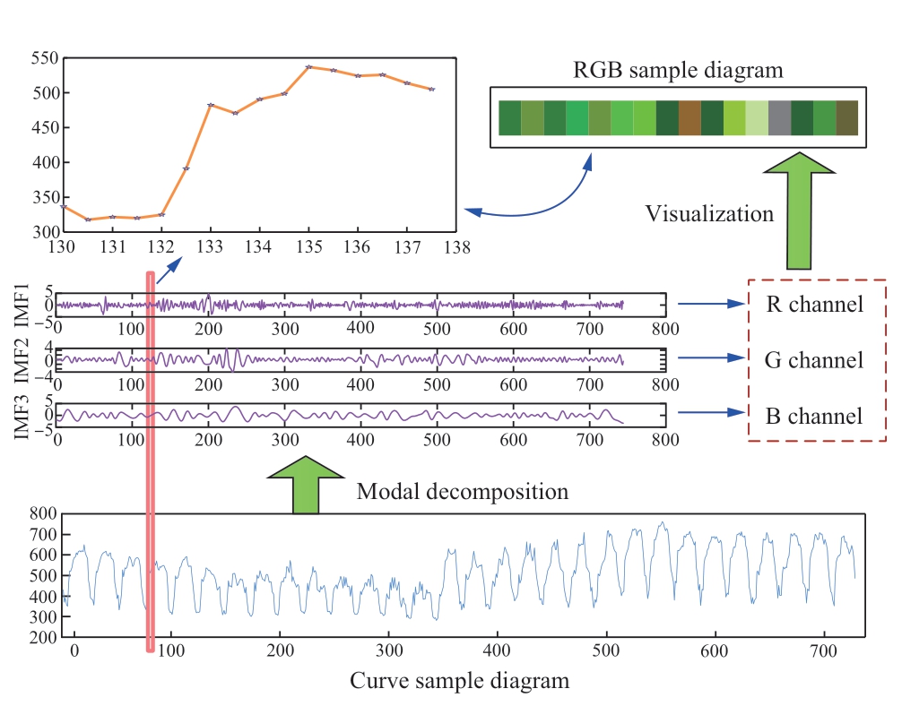
Fig.4 Reciprocal diagram of RGB image and load curve

2.3 DenseNet and its optimizations

DenseNet is an improvement of the convolutional neural network,which can maximize the data characteristics,reduce the number of required parameters,and achieve better processing results.The DenseNet network structure comprises DenseBlock,Convolution,Transition,Pooling,Linear,and Softmax functions,as shown in Fig.5.

Fig.5 DenseNet structure chart

The function of the convolutional layer is to select the size and number of convolution kernels,and the function of the pooling layer is to reduce the size of the image,which can effectively smoothen the image and denoise.DenseBlock is a new concept,and DenseBlocks are stacked to form a DenseNet,as shown in Fig.6.Each DenseBlock in the figure contains five DenseLayers.The DenseLayer is composed of a convolutional layer and a pooling layer.x0 is used as the input image to obtain the image x1 through the function H.On the channel dimension,x0 and x1 are connected by a cat and become the input of the next H function.Accordingly,cascade the output feature maps of each layer.Each DenseBlock is connected with a transition layer,which can change the number of channels of the feature map,that is,the number of channels of each RGB image is three.To reduce the network load,a bottleneck layer (1×1 convolution) is added before the convolution operation to improve the computing efficiency of the network.Finally,the image passes through the last DenseBlock into the final pooling layer,Linear layer,and Softmax function,and outputs the classification label.

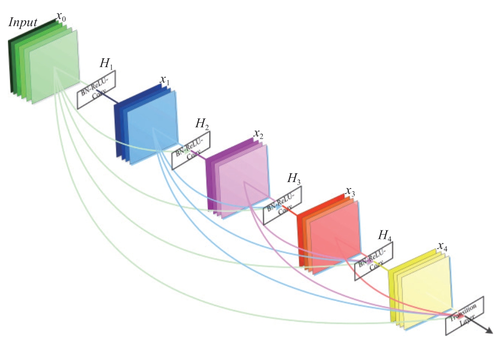
Fig.6 Dense Block structure chart

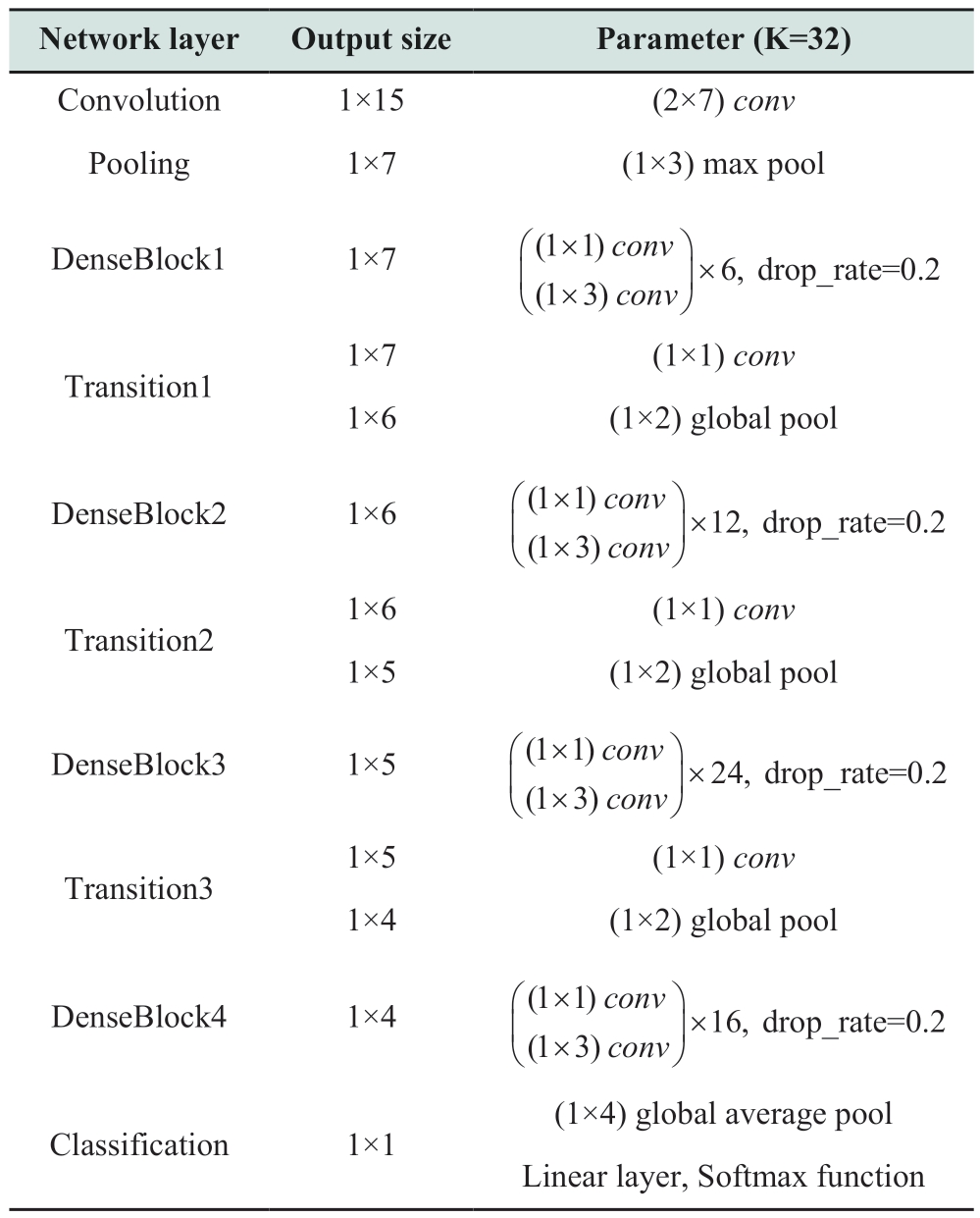
On the basic DenseNet network [19,20],four improvements were made in this study,labeled DenseNet-A(B,C,D).The difference between each network is the number of DenseBlocks and DenseLayers.In comparison,DenseNet-A is more effective.The data image size used to describe the DenseNet-A network structure is 2 × 30 × 3(rows × columns × channels).

The network structure of DenseNet-A is presented in Table 2,where conv refers to the BN-RELU-CONV layer that includes batch normalization (BN) and ReLU functions.Following the convolution operation,it passes through a BN-RELU-CONV layer.The number of channels increases by k for each DenseLayer passed.For example,after the first convolutional layer,the number of channels increases from 3 to 64.To remove some neurons in the network,a dropout layer is added after the DenseLayer,which fully inhibits overfitting [21].The dropout rate in the table represents the probability of removal.DenseNet-A contains four DenseBlocks,and the number of DenseLayers in each DenseBlock is (6,12,24,and 16).

Table 2 DenseNet-A network structure

3 Diversified image processing methods

Generalized load data are unpredictable,and their trends include unimodal type,bimodal type,and other situations,making it difficult to predict the generalized load.This study used a 3-year dataset for training.The number of images were generated by the training set is approximately 2880 images in a time window of 30 days.This capacity is low for DenseNet-A and training a small dataset with a large neural network creates two problems.First,the network model cannot learn the general mapping relationship between the input and output,which reduces its generalization ability and results in poor performance for new datasets [22,23].Second,for the relationship between the input space structure and its output,a small dataset provides less descriptive information,which leads to the oscillation and discretization of the input space,and it is difficult to learn feature mapping.

3.1 Gaussian diversification processing

To solve the problems of the poor generalization ability of the model and discrete oscillation of the input space,Gaussian noise (GN) can be added to the data image using the Gaussian diversification processing method to achieve the effect of smoothing the input space structure.The smoothing effect makes it easier for a network to learn the feature mapping [24].

When Gaussian noise is added,the signal-to-noise ratio of the parameter is particularly important,and it is difficult to achieve its effect if the ratio is too large or too small.Select the pixels (i,j) and (i,j+1) adjacent to the left and right of the image data to generate two random numbers r and φ between [0,1],In this study,the signal-to-noise ratio (snr=6)is selected,and the Gaussian noise is calculated as follows:

where GN1 and GN2 are the noise values of each pixel in the first and second rows of the image,respectively.According to (4),the noise value that corresponds to each pixel in a certain row of images can be obtained,and the pixel value (PV) after adding noise can be obtained by adding the pixel value to the pixel value at the original position.

The pixel value of the image in the third row was obtained by adding noise to the basic data image in the first row.The reverse basic data from the second row produced the fourth row of images.The same generation method was used in the present study.The result of (5) is added to the Gaussian noise to form a new line of images and then the resulting image data are normalized:

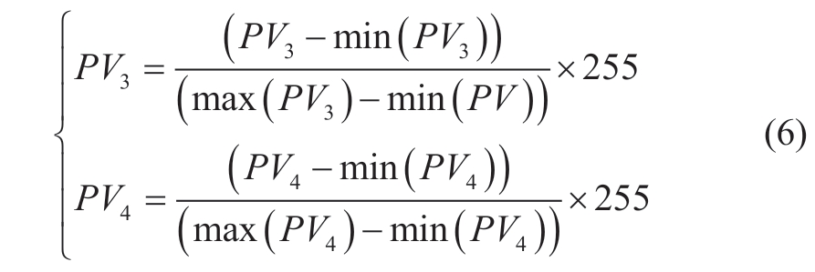
Following the normalization process of (6),the pixel values are in the interval [0,255],and the third and fourth rows of the image data are formed by adding Gaussian noise to the first and second rows,as shown in Fig.7.

Fig.7 Gaussian diversity processing sample diagram

3.2 Reverse diversification processing

To add data,the reverse was selected to process the original data and add them to the second row of the data image.Reverse diversification is the reversal of upward and downward ranges.In numerical calculations,reverse processing involves changing the rise of ＞1 to a fall of ＜1,and vice versa.Reverse diversification does not change the original data image but only increases the image information.The image is increased from one line to two lines,as shown in Fig.8.

Fig.8 Reverse diversification processing sample diagram

4 Case study

4.1 Basic data

To solve the problem of the lack of analysis data for generalized loads,this study generates data for future generalized loads based on an established simulation model.Subsequently,the density-based DBSCAN clustering algorithm was used to extract feature curves from the generalized load data.Finally,the characteristic curves of the generalized loads under different scenarios were simulated and analyzed,and various generalized load characteristic curves were obtained.Concurrently,the prediction effect of the prediction method adopted in this study can be verified under different generalized load scenarios.

Grid-base load data were selected as the ISO New England load data from February 1 to September 30,2022.The DBSCAN algorithm is used to cluster the underlying data.The characteristic curve of the selected load is the central curve of each cluster,as shown in Fig.9 (a).The characteristic curves of the base load exhibit three typical patterns: the first category is unimodal,and the second and third categories are bimodal.

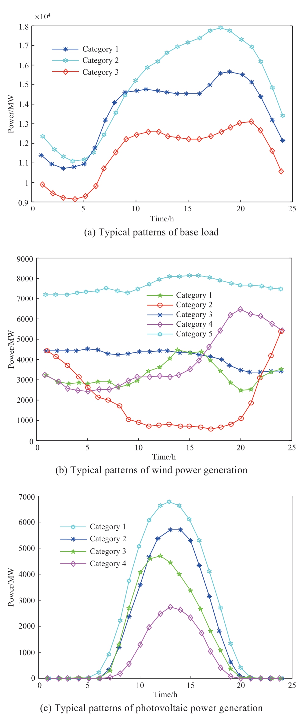
Fig.9 Characteristic cure of base load,wind power,and photovoltaic generation curve

The new energy power generation data were based on wind and photovoltaic power generation data from the German company Tennet from February 1 to September 30,2022.The characteristic curves of wind and photovoltaic power generation were also extracted using the DBSCAN clustering algorithm,and the extraction results are presented in Fig.9 (b) and Fig.9 (c).In Fig.9 (b),significant differences exist between the typical wind power patterns.For example,the typical Type 1 pattern had a higher output level during the day than at night,while the typical Type 3 pattern shows the opposite pattern.In Fig.9 (c),the peak period of the output of various typical photovoltaic patterns is within the 10-14 h time period.Based on the extraction results in Fig.9,the difference between the feature curves extracted by the DBSCAN clustering algorithm is evident,and the extraction effect is better.

The generalized load PGL,re considering the access of new energy is calculated as follows:

where Pbase denotes the base load of the power grid and Pre indicates the power vector of the new energy generation.When new energy sources with different permeabilities are accessed,PGL,re can be obtained under different scenarios.

According to (7),the generalized load characteristic curves under different proportions of renewable energy access can be obtained,as shown in Fig.10.

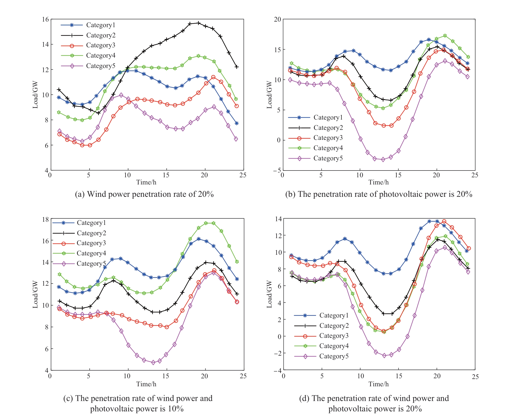
Fig.10 Characteristic curves of generalized load in scenarios with different permeabilities of renewable energy

Fig.10 (a) depicts the scenario with a wind power permeability of 20%,and the generalized load characteristic curve includes five types.Among them,Types 1,2,3,and 5 are all bimodal,whereas Type 4 is unimodal.Access to wind power makes load changes more complicated,and the uncertainty of the load increases,which causes certain difficulties in the planning and dispatching of the power grid.

Fig.10 (b) shows a scenario with a photovoltaic permeability of 20%.The typical pattern of a generalized load characteristic curve is a depression in the middle of the curve.Since the curve of photovoltaic power generation curve presents a typical single peak with light intensity,the load curve has a large trough value at noon.Additionally,the trough value of load curve Category 5 in the figure is negative because,at this time,photovoltaic power generation supplies power to the grid,and the grid cannot fully absorb it,so it can be sent out.Fig.10 (c) shows the scenario when wind and photovoltaic power generation are connected simultaneously,and the wind and photovoltaic permeabilities are both 10%.The load characteristic curves of wind and photovoltaic power generation simultaneously connected to the grid are more complex than when the two are connected separately.Figure 10 (d) shows the wind and photovoltaic permeabilities at 20%.The characteristics of the typical generalized load pattern in this scenario are similar to those in Fig.10 (b),when photovoltaic power generation is connected with large troughs at noon.

Generally,the typical patterns of the generalized load under the different scenarios shown in Fig.10 are divided into five categories.By comparing Fig.9 (a),it can be observed that the access of different proportions and types of renewable energy leads to complexity of the generalized load curve pattern.Therefore,it is necessary to consider the curve characteristics of a generalized load when planning the operation of a power grid,including wind and photovoltaic power generation.

4.2 Modal decomposition of generalized load data

Once the generalized load scenario was established,the load time series was decomposed.Load time series often contain a large number of high-frequency components,are highly nonlinear,and are not sufficiently smooth,which significantly increases the difficulty of forecasting and reduces its accuracy.Therefore,one way to solve this problem is to decompose the load time series into a series with strong smoothness and low complexity.The CEEMDAN can decompose a load time series into IMF components with different types of information.CEEMDAN does not directly add the Gaussian white noise signal to the original signal,but averages the modal components obtained by EMD decomposition as a whole and then CEEMDAN decomposition calculates the overall average after obtaining the first-order IMF components to obtain the final first-order IMF components.This process is repeated for the residuals.This effectively solves the problem of white noise shifting from high to low frequencies.

Considering the generalized load data under a wind power permeability of 20% as an example,three sets of IMF are obtained using the CEEMDAN to decompose the generalized load for one month,as shown in Fig.11.

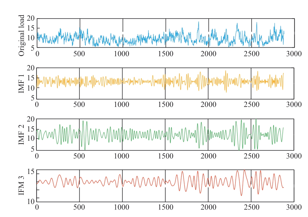
Fig.11 Load data for CEEMDAN decomposition

The distribution of frequencies from high to low can be observed,and the data complexity is significantly reduced compared with the original load time series.The CEEMDAN algorithm improves both the reconstruction accuracy and decomposition efficiency.

4.3 Visualization and diversified processing of generalized load data

The obtained generalized load data are visualized and diversified based on the two diversification methods proposed in Section 3.The data were used to evaluate the effectiveness of the two diverse predictions.The comparison results are presented in Fig.12.

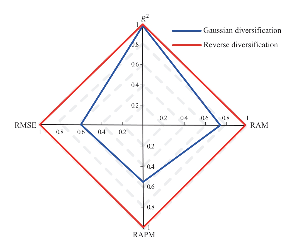
Fig.12 Comparison of error indexes obtained with different processing methods

In Fig.12,by comparing the error indexes of the two diversification predictions,it can be observed that the error indexes after the reverse diversification process are improved compared with the Gaussian diversification,and the difference is obvious.This indicates that added diversity information is more useful after the image is inversely diversified.However,the manner in which Gaussian diversification increases diversity does not satisfy the proposed prediction method.From the above results,it can be concluded that Gaussian diversity increases the diversity of images,but the utilization rate of information is low,and more useless information affects the judgment of the network.Most of the feature information learned by the network for this problem is ineffective,and its optimization effect is poor.For the generalized load-forecasting problem in this study,the predictive effect of reverse diversification is better than that of Gaussian diversification.

4.4 Results and analysis of generalized load forecasting

Through data processing,modal decomposition,load data visualization,reverse diversification processing,and DenseNet neural network optimization,sufficient preparations were made for the load forecasting.Subsequently,the optimized DenseNet-A neural network was used to make short-term predictions of the generalized load data under the different permeabilities of wind and photovoltaic power generation selected in Section 4.1.The RGB image prediction results for the load data are converted into load curves,as shown in Fig.13.

 

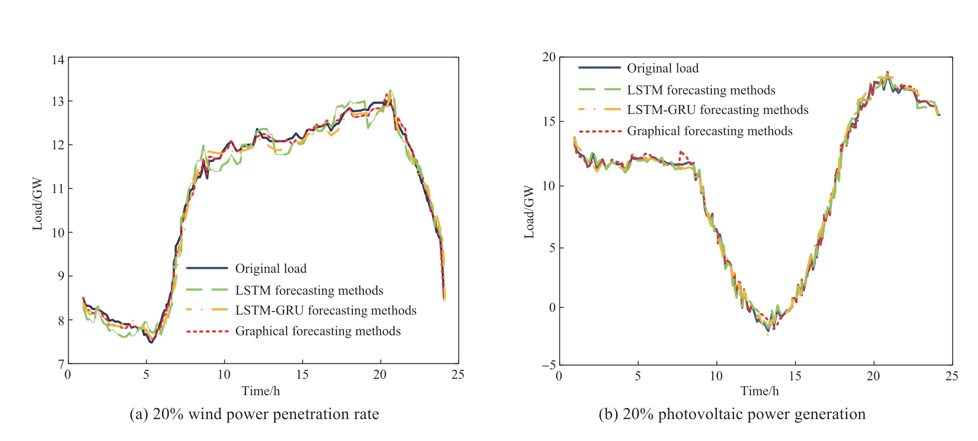
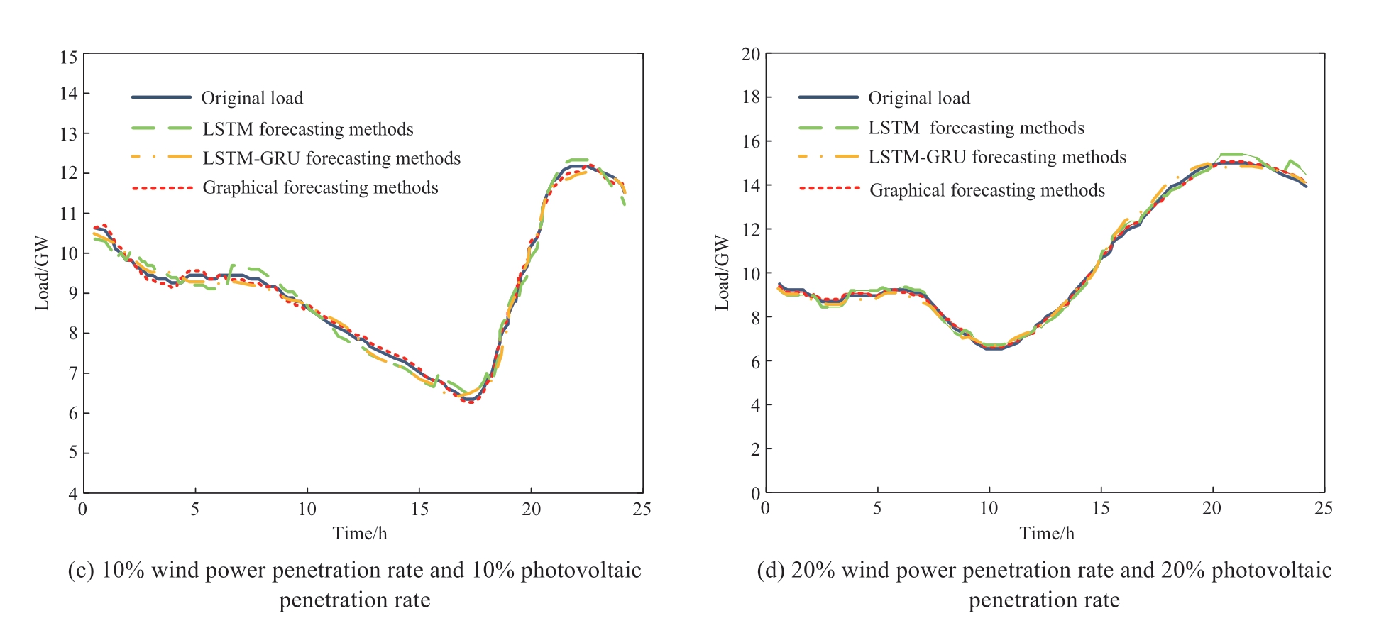
Fig.13 Forecasting results under different generalized load scenarios

The results of the graphical forecasting method are compared with those obtained by the traditional LSTM and LSTM-GRU load curve forecasting methods,and the feasibility of the method is illustrated [9,25,26].The error indicators after comparison are listed in Table 3.

Table 3 Predictive evaluation indicators of different models

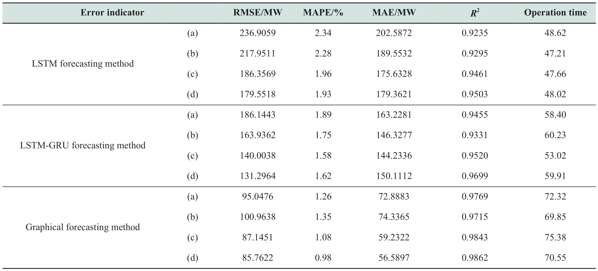
As indicated in Fig.13 and Table 3,the prediction results obtained in the four scenarios are better than those of the traditional LSTM neural network load sequence prediction method,and the prediction accuracy is improved.Compared with the scenario where the permeabilities of wind power and photovoltaic power are 10% and 20%,respectively,the graphical prediction method has a better prediction effect in the scenario of wind power permeability of 20% or photovoltaic power permeability of 20%.It can be concluded that the proposed method is suitable for generalized load forecasting in complex scenarios with a high proportion of renewable energy access,and the feasibility of the method is verified.Additionally,although the model proposed in this study is more complex than the traditional model and requires a long operation time,it can improve the accuracy of load prediction and verify the feasibility of the model.

5 Conclusion

In this study,we proposed a graphical short-term prediction method for generalized loads based on modal decomposition.In the proposed method,the generalized load data under different permeabilities of wind and photovoltaic power generation were converted into RGB images by modal decomposition.Through visualization and reverse diversification processing,the feature information of various types of generalized loads were fully mined,and good prediction accuracy was obtained.DenseNet-A was used for training and prediction,and the advantages of the proposed method over the traditional load series prediction method were verified through a case analysis.The proposed method provides a new approach for predicting generalized loads.In the future,the coupling effects of multiple factors,such as electric vehicle charging and discharging,and the demand-side response will be comprehensively considered to improve the comprehensiveness and accuracy of generalized load research.

Acknowledgements

This study was supported by the National Natural Science Foundation of China (Grant No.62063016).

Declaration of Competing Interest

We declare that we have no conflicts of interest.

References

[1] Tan X D,Liu J,Xu Z C,et al.(2021) Power supply and demand balance during the 14th five-year plan period under the goal of carbon emission peak and carbon neutrality.Electric Power,54(5): 1-6(in Chinese)

[2] Jia S L,Xiao X Y,Zhou K (2023) Column review:Environmentally-friendly power equipment for the dual carbon goal.Advanced Engineering Sciences,55(04): 1-2

[3] Mohammadi A,Mehrpooya M (2018) A comprehensive review on coupling different types of electrolyzer to renewable energy sources.Energy,158: 632-655

[4] Abdin Z,Zafaranloo A,Rafiee A,et al.(2020) Hydrogen as an energy vector.Renewable and Sustainable Energy Reviews,120:109620

[5] Kaur A,Nonnenmacher L,Coimbra C F M (2016) Net load forecasting for high renewable energy penetration grids.Energy,114: 1073-1084

[6] Li J H,Lai C W,Chen B,et al.(2019) Research concept of pattern features of generalized load curves in future power systems.IEEE Innovative Smart Grid Technologies-Asia (ISGT Asia),May 21-24,Chengdu,China: 1-5

[7] Li J H,Lei Y S,Huang Q,et al.(2019) Feature analysis of generalized load patterns considering active load response to realtime pricing.IEEE Access,7: 119443-119453

[8] Deng D Y,Li J,Zhang Z Y,et al.(2020) Short-term electric load forecasting based on EEMD-GRU-MLR.Power System Technology,44(2): 593-602 (in Chinese)

[9] Eskandari H,Imani M,Moghaddam M P (2021) Convolutional and recurrent neural network based model for short-term load forecasting.Electric Power Systems Research,195: 107173

[10] Zhang Y H,Robert Q,Yang F,et al.(2019) Overview of application of deep learning with image data and spatio-temporal data of power grid.Power System Technology,43(06): 1865-1873

[11] Zhang Y H,Yang F,et al.(2019) Overview of application of deep learning with image data and spatio-temporal data of power grid.Power System Technology,43(6): 1865-1873(in Chinese)

[12] Yang Y L,Qi L H,Wang H,et al.(2020) Reconstruction of missing measurement data in distribution network based on generative adversarial network and double semantic perception.Automation of Electric Power Systems,44(18): 46-54(in Chinese)

[13] Wang H,Qi L H,Yan L,et al.(2021) Load photo: A novel analysis method for load data.IEEE Transactions on Smart Grid,12(2): 1394-1404

[14] Ji J,Jiang Z,Yin X,et al.(2022) Slope reliability analysis based on deep learning of digital images of random fields using CNN.Chinese Journal of Geotechnical Engineering,44(08): 1463-1473(in Chinese)

[15] Li S S (2020) An improved DBSCAN algorithm based on the neighbor similarity and fast nearest neighbor query.IEEE Access,8: 47468-47476

[16] Xia D W,Bai Y,Zheng Y L,et al.(2022) A parallel SPDBSCAN algorithm on Spark for waiting spot recommendation.Multimedia Tools and Applications,81(3): 4015-4038

[17] Lee J,Sun Y G,Sim I,et al.(2022) Non-technical loss detection using deep reinforcement learning for feature cost efficiency and imbalanced dataset.IEEE Access,10: 27084-27095

[18] Liu X,Yang X Q,Zhu P B,et al.(2021) Robust multimodel identification of LPV systems with missing observations based on t-distribution.IEEE Transactions on Systems,Man,and Cybernetics: Systems,51(8): 5254-5260

[19] Lai G K,Chang W C,Yang Y M,et al.(2018) Modeling long and short-term temporal patterns with deep neural networks.The 41st International ACM SIGIR Conference on Research &Development in Information Retrieval.Ann Arbor: ACM,95-104

[20] Xu Z H,Ma W,Lin P,et al.(2022) Deep learning of rock microscopic images for intelligent lithology identification: Neural network comparison and selection.Journal of Rock Mechanics and Geotechnical Engineering,14(04): 1140-1152

[21] Zhao Y Q,Song Y Q,Wu H,et al.(2023) High-precision gesture recognition based on DenseNet and convolutional block attention module.Journal of Electronics &Information Technology,1-10

[22] Ji Z W (2022) Dropout optimization of neural network over fitting problem.Journal of Changzhi University,37(2): 37-39

[23] Niu R X,Ding H,Shi R,et al.(2022) Rolling bearing fault diagnosis method based on improved densely connected convolution network.Journal of Vibration and Shock,41(11):252-258(in Chinese)

[24] Zhong Y,Zhao M (2020) Research on deep learning in apple leaf disease recognition.Computers and Electronics in Agriculture,168: 105146

[25] Majed H E,Sabine S (2020) Blind universal Bayesian image denoising with Gaussian noise level learning.IEEE transactions on image processing: a publication of the IEEE Signal Processing Society,294885-4897

[26] Guo H Y,Chen Q X,Zheng K D,et al.(2021) Forecast aggregated supply curves in power markets based on LSTM model.IEEE Transactions on power systems,36(6): 5767-5779

[27] Tang Y,Wang Y,Duan S,et al.(2023) Fault diagnosis of the LAMOST fiber positioner based on a long short-term memory(LSTM) deep neural network.Research in Astronomy and Astrophysics,23(12): 83-97

Scan for more details

Recieved: 2 January 2024/Revised: 5 March 2024/Accepted:8 March 2024/Published: 25 April 2024

Lizhen Wu

wulzlut@163.com

Peixin Chang

3057342712@qq.com

Wei Chen

17693100904@163.com

Tingting Pei

peitt52@163.com

2096-5117/© 2024 Global Energy Interconnection Development and Cooperation Organization.Production and hosting by Elsevier B.V.on behalf of KeAi Communications Co.,Ltd.This is an open access article under the CC BY-NC-ND license (http://creativecommons.org/licenses/by-nc-nd/4.0/).

Biographies

Lizhen Wu received the M.S.degree in the control theory and control engineering from Lanzhou University of Technology,Gansu,China,in 2004,and Ph.D.in control theory and control engineering from Lanzhou University of Technology in 2017.She is studied power systems and automation at the National Active Distribution Network Technology Research Center,Beijing Jiaotong University,Beijing,China,in 2015.Currently,she is an Associate Professor/Master Supervisor at the College of Electrical and Information Engineering,Lanzhou University of Technology,where she teaches courses on power electronics,control theory,and renewable energy systems.Her interests include distributed generation and microgrids,microenergy grid coordination control,power quality control,artificial intelligence and style="vertical-align: middle; text-align: center;">