0 Introduction

In recent years, fossil fuel depletion and environmental pollution have become major social development problems [1].The emergence and development of renewable energy power generation provide an opportunity to solve these problems. An integrated energy system (IES) is important for the development of an energy internet [2]. An IES is primarily based on a power system as the fundamental framework. It couples electricity, gas, heat, and other energy forms to achieve stepped use. It draws upon the complementarity of various heterogeneous energy sources, improves resource utilization efficiency [3, 4], and reduces carbon dioxide emissions. As the penetration of renewable energy increases, the energy output fluctuates and is random, posing a considerable challenge to system operation [5]. Consequently, dealing with the uncertainty of renewable output and considering both economic and environmental objectives have become a research focus.

Currently, the power-to-gas (P2G) technology, which connects power and natural gas systems that convert electricity into natural gas, reduces carbon emissions. In [6],the essence of carbon capture systems (CCSs) involved the production of CO2 capture and storage units using various methods to avoid CO2 entry into the atmosphere and reduce large-scale CO2 emissions [7]. In [8], an integrated energy reduction unit (IEPU) system that combined P2G and CCS technologies was proposed. The CO2 captured by the CCS was converted into natural gas, and the coupling characteristics of electricity, heat, gas, and carbon were analyzed [9]. Hydrogen is an important decarbonization pathway for the development of energy interconnections.Based on the CCS-P2G coupling system, considering the two-stage process of P2G, a comprehensive model of CCS and HFC was proposed in [10]. Experimental results showed that the CO2 emissions and operating costs of the IES were reduced. Based on the carbon trading mechanism,a hydrogen-based IES (HIES) operation framework was established to improve the P2G system and CCS [11, 12].In [13], a wind-photovoltaic (PV)-load-hydrogen system model was established. The model provided an effective means for enabling the renewable energy of the IES to adapt to a reliable hydrogen supply. The foregoing research mainly focuses on the carbon reduction analysis of the energy production side; the demand-side resources also have considerable carbon reduction potential [14, 15]. Considering the thermal inertia of buildings and the economic benefits to users, a IES bilevel optimal scheduling model was formulated in [16] using an acceptable temperature range to satisfy the thermal comfort requirements. Multienergy users actively obtain retail energy price signals and formulate optimal multi-energy use strategies [17, 18].In [19], an integrated electricity-gas system architecture for the coordinated operation of source-side P2G, CCS,and load-side electric vehicles was proposed. The system has satisfactory economic benefits and environmental friendliness. Further, the combination of source and demand scheduling is considered in [20]. In view of the foregoing problems and multiple uncertainties, a distributionally robust optimization model based on Wasserstein and multivariate linear affine was proposed in [21]. A few studies have been conducted on the operational optimization of energy systems. The studies accounted for the uncertainty of new energy outputs combined with the utilization of source-side hydrogen energy and the invocation of load-side resources for bilateral collaborative carbon reduction.

The uncertainty of wind power and PV output severely affects operational economy. In recent years, scholars have gradually focused on using historical output data containing uncertainty information. These data are used to construct prediction error probability density distributions, provide probability interval predictions, and establish distributionally robust optimization models [22-24]. Probability density estimation calculates the overall probability density function through samples; it is typically divided into parametric and nonparametric forms. In [25], a mixed Weibull model is used to estimate the probability densities of wind speed and wind energy to study the distribution characteristics of wind energy resources. Based on the statistical information on wind power, the kernel density estimation method was used to model the uncertainty of the wind power output.The distribution characteristics of wind power data were accurately described, and a model of the probability distribution fuzzy set was constructed. To determine the influence of the bandwidth selection of kernel density estimation on error estimation results, a probability density distribution of the wind power prediction error was proposed in [27]. The distribution was based on nonparametric kernel density estimation, which could improve the fitting of the prediction error of wind power. Then, an accurate confidence fluctuation domain of wind power can be constructed. Kernel density estimation accurately indicates that the output error information must be precise in the statistical data with no outliers. To solve this problem,[28, 29] proposed a robust kernel density estimator (RKDE)to weaken the influence of outliers on the probability density and improve the accuracy of the probability density estimation. Although this method assigns a weight to each kernel function to weaken the influence of outliers on the probability distribution, it uses a fixed smoothing parameter for the estimation of wind and solar outputs. Moreover,the distribution cannot be better fitted with the change in observed values. To resolve this problem [30], a variable bandwidth that can achieve higher accuracy than that the bandwidth used in traditional methods was found.

The main contributions of the study considering two aspects are summarized as follows.

1) An improved RKDE (IRKDE) is proposed to weaken the influence of outliers, construct the distribution information of wind and PV outputs, and construct a datadriven uncertainty set based on the distribution information.

2) A source-load collaborative robust optimization model for comprehensive demand response is established.The model considers the two-stage process of combined heat and power (CHP), CCS, and P2G; the further utilization of energy using hydrogen energy coupling equipment on the source side; and the flexibility of schedulable resources on the load side.

This paper is organized as follows. The composition and modeling of CHP-CCS-P2G are described in Section 1. The construction of the source-load model is presented in Section 2. Section 3 elaborates on the constraints and scheduling objectives of an IES and its robust forms. The simulation analysis is presented in Section 4. Finally,Section 5 summarizes the conclusions.

1 Structure and model construction of HIES

1.1 Composition of HIES coupling equipment

The composition of the HIES coupling equipment is shown in Fig. 1. It includes the following: PV, wind turbine(WT) units, CHP, gas boiler (GB), electric boiler (EB),CCS, electrolytic cell (EL), carbon storage (CS), methane reactor (MR), hydrogen fuel cell (HFC), hydrogen energy storage (HES), electric energy storage (EES), thermal energy storage (TES), and integrated demand response load of electricity, heat, and gas.

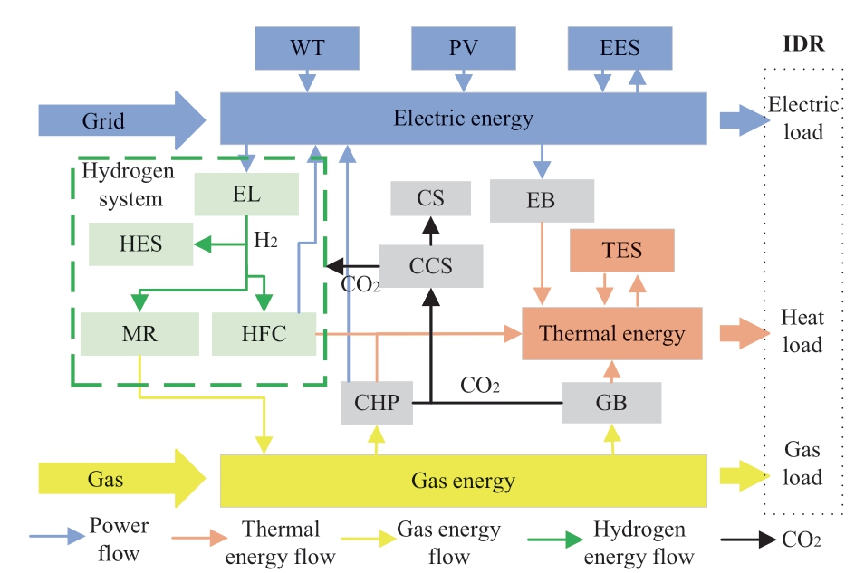
Fig. 1 Composition of comprehensive energy system containing hydrogen energy

1.2 CHP-CCS-P2G

The modeling of the P2G two-stage process is considered. The CCS captures the CO2 generated by the CHP and GB equipment that burns natural gas as well as directly uses and stores it. This avoids the cost and risk of H2 long-distance transportation and CO2 storage. The hydrogen produced by water electrolysis in the two-stage process of CO2 capture by CCS and P2G can solve the problem of using raw materials in the methanation process to synthesize CH4. Moreover, the two-stage process can fully utilize hydrogen energy, reduce system operating costs, reduce environmental pollution, and improve the utilization of clean hydrogen energy. The specific model is as follows:

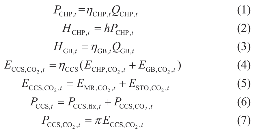
where PCHP,t, HCHP,t, and h are the CHP output electric power,thermal power, and thermoelectric ratio, respectively;QCHP,t and QGB,t are the CHP and GB natural gas power consumptions, respectively; HGB,t and ηGB,t are the GB output thermal power and heating efficiency, respectively; ECCS,CO 2 ,t and ηCCS are the amounts of CO2 captured by the CCS and the capture efficiency, respectively; ECHP,CO 2 ,t and EGB,CO 2 ,t are the amounts of CO2 produced by the CHP and GB units,respectively; ESTO,CO 2 ,t is the CO2 storage; PCCS,t, PCCS,fix,t,and PCCS,CO 2 ,t are the operational energy consumption,fixed energy consumption, and carbon capture energy consumption of the CCS, respectively; and π is the power consumption per unit of CO2 treatment.

The P2G two-stage process considers the utilization of hydrogen energy. Electrical energy is converted into H2 by ELs consuming electrical energy, rendering the P2G process more flexible and improving energy efficiency. The methanation process synthesizes CH4 by consuming CO2 and H2. Hydrogen can also serve as a fuel base for HFCs.The specific output model is as follows:

where PEL,H 2 ,t and PEL, e ,t are the hydrogen production power and input electric power of the EL, respectively; Lgas is the calorific value of natural gas; PMR, g ,t, ηMR, and EMR,H 2 ,t are the natural gas power, operating efficiency, and hydrogen consumption generated by the MR, respectively; and κ is the gas mass per cubic meter of the natural gas pipeline.

Because the volume of CO2 required for the methanation of hydrogen is equal to the volume of CH4 produced by methanation, the mass of CO2 required for methanation is given by Equation (10):

where EMR,CO 2 ,t is the amount of CO2 consumed in the methanation process, and ρCO2 is the CO2 density.

An HFC device is introduced. This fuel cell converts hydrogen energy into electric and heat energies by consuming H2. It decouples hydrogen energy from the electric and heat energies and improves the clean energy utilization rate in the IEPU. The model is as follows:

where ηHFC,e and ηHFC,h are the electricity generation and thermal efficiency of the HFC, respectively. Moreover,PHFC,H 2 ,t, PHFC,t, and HHFC,t are the consumed hydrogen,electricity, and heat power produced by the HFC,respectively.

The EB, power storage, and heat storage device models are described in detail in the literature [31].

1.3 Integrated demand response

1) Flexible electrical and gas loads

In general, the fluctuation in daily load is consistent with the peaks and valleys of the time-sharing energy price. Therefore, the demand price elasticity coefficient is introduced to describe the relationship between user demand and energy price. Equations (13) and (14) represent the amount of load reduction and transfer of the user demand response for energy prices, respectively; k denotes the k types:

where k = {e,g}; ∆Pk (t ) and ∆Pk 0( t) are the k-load variation and initial load at moment t, respectively; ∆ρk ,t and are demand response and initial prices, respectively;∆Pk CL(t ) and ∆Pk SL(t ) are the amounts of load reduction and transferable load after demand response, respectively;PkCL,0(t ) and PkSL,0( t) are the initial reducible load and initial transferable load, respectively; and ρk ,t represents the time (t)demand response energy at price k.

2) Flexible heat load

Considering that the thermal user’s perception of the change in ambient temperature is ambiguous, a fixed heating load can be converted into a heating load interval to provide greater flexibility for the system. The predicted mean vote (PMV) is introduced to evaluate the comfort of the indoor thermal environment [18].

Considering that the daytime and nighttime activities of users are inconsistent (i.e., the thermal comfort of users varies), this study limits the load-all-day PMV values.Therefore, the heat demand relationship considering the thermal comfort elasticity is

where Ph ,t ,min and Ph ,t ,max are the minimum and maximum total heat load demands for satisfying the load thermal comfort elasticity in time t, respectively. Moreover,

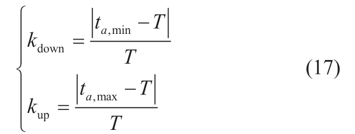
where kup and kdown are the heating elasticity coefficients; T denotes the daily standard heating ambient air temperature expected by the user (24 °C in this study); and ta,min and ta,max denote the minimum and maximum boundary values of room temperature accepted by the user, respectively.

Considering thermal load elasticity of the user, the overall heat demand during the user’s scheduling cycle must be consistent with the heat demand before considering thermal load elasticity. This avoids affecting the user demand for thermal load throughout the day.

2 Uncertainty source-load modeling

2.1 Improved kernel density estimation

In the current research, a kernel density estimation(KDE) is typically used to estimate the uncertainty of renewable energy outputs. However, its disadvantage is that kernel density is sensitive to data outliers. Typically, this leads to an overestimation of the true probability density.Accordingly, a weighted RKDE is proposed. This method assigns a weight value to each kernel function to weaken the effect of outliers on probability distribution.

Suppose that F and f are the probability distribution and probability density function of the uncertainty parameters,respectively, and ζ1, K, and ζN are N samples from distribution F. The probability kernel density estimation of f has the following form:

where Kσ is the kernel function, and r( ) is the probability density function. In this study, the Gaussian kernel density function is selected. The foregoing model can be rewritten as a robust Gaussian kernel density estimation function, as follows:

The number of weighting parameters is N, and

Although the forgoing robust kernel density assigns a weight value to each observation, it weakens the influence of outliers on the probability density. The selection of kernel density estimation parameters directly affects the density estimation results. The selection process for weight calculation and smoothing parameters is described below.This study improves the basis of a robust kernel density and selects appropriate smoothing parameters for each observation value to achieve an effective estimate of the real density function.

1) Weight calculation

In this study, the kernelized iteratively reweighted least squares method [30] is used to calculate the weight of the function:

where Φ(ξ )=Kσ (•, ξ), and H reproduce the kernel Hilbert spaces generated by Φ(ξ ). Moreover, ϕ is a robust loss function (the loss function is the most significant difference between the RKDE and KDE methods). The Humpel loss function is used in this study.

To obtain ( )ξ , the initial weighti=1, …,N ) is repeated to iterate the weight of the estimation function such that the latest estimation function can approximate the true density function obtained by substituting the observed value.

2) Adaptive robust kernel density smoothing parameters

Robust kernel density estimation adopts a global fixed smoothing parameter. In practical applications, ensuring that the smoothing parameter calculated using this formula is the optimal solution is difficult. The data at both ends of the extreme values of the dataset are possibly highly dispersed, whereas the central data are less dispersed,affecting the overall fitting. Therefore, to analyze the fitting effect further, the global fixed smoothing parameters are improved. Moreover, a robust kernel density estimation of the adaptive smoothing parameters is proposed. The function corresponding to each observation value selects different smoothing parameters such that the estimation function fitting further approximates the real density function.

After obtaining the fixed smoothing parameters, the distance between all intervals and k adjacent intervals is calculated using Equation (21):

where αk is a constant, and di ,k is the Euclidean distance between the observed value and its nearest k neighbor.Compared with the kernel density of the fixed smoothing parameter, the adaptive smoothing parameter, σi, is used to change the influence distance of the probability density estimation through the adaptive factor according to the probability of existing data sample points. The extreme values at both ends with large dispersion expand the bandwidth. In contrast, the central data with small dispersion reduce the bandwidth. This can effectively solve the problem of boundary deviation and lack of local adaptability, thus improving the accuracy and adaptability of the probability distribution of uncertainty sets.

By connecting the foregoing to robust kernel density estimation (RKDE), the following is obtained:

2.2 Renewable energy output range

Assume that ui is an uncertainty quantity. The cumulative distribution probability function is obtained for(u i ), and the quantile function is defined as

Therefore, an uncertainty set with confidence level(1 − 2 )α can be obtained:

2.3 Establishment of random load scenario

In this study, stochastic scenario analysis technology is used to resolve the uncertainty of electrical, thermal, and gas loads. First, according to the probability distribution of the predicted error value of each load, the Latin hypercube sampling method is used to simulate and generate multiple scenarios of each load in the prediction error interval.Typical scenarios of electrical, thermal, and gas load energy consumptions are obtained by combining scenario reduction technology [32].

The probability distribution of the prediction errors of the electrical, heat, and gas loads is normal. First, based on the prediction error probability distribution for each load,multiple scenarios for each load in the prediction error interval are simulated using the Latin hypercube sampling method. Then, typical scenarios for each load are obtained using the fast backward reduction method. The numbers of electrical, heat, and gas load scenarios obtained at this time are set as κe, κh, and κq, respectively, and the probabilities of each scenario are set as πe, πh, and πq, respectively. The total number of load scenarios, S, and the probability of each scenario, π, obtained by the optimization calculation in the scheduling model are as follows:

3 id="generateCatalog_12" style="text-align: left; text-indent: 0em; font-size: 1.2em; color: rgb(195, 101, 0); font-weight: bold; margin: 0.7em 0em;">3.1 Objective

The IES considering the operation of hydrogen energy coupling equipment accounts for the operation and maintenance cost of each piece of production capacity equipment, energy coupling equipment, energy storage device (f1), energy purchase and sales cost ( f2), carbon cost( f3), and penalty cost ( f4):

where πs is the probability of scene occurrence.

1) The operation and maintenance costs are given by

where mi and nk are the maintenance costs of the ith energy coupling equipment and k energy storage equipment,respectively. Moreover, Pi ,t, , and  are the i coupling device output, energy storage charging, and energy storage discharging, respectively.

2) The energy purchase and sales costs are given by

where , , and  are the electricity purchase,electricity sale, and gas purchase prices, respectively.Furthermore, , , and represent the power purchase, power sale, and gas purchase power, respectively.

3) The carbon cost is obtained as follows:

where rCO2 and rSTO are the carbon emission trading and CO2 storage cost coefficients, respectively. Moreover, Ep ,a , Ep,and ESTO,CO 2 ,t are the initial carbon quota, actual carbon emission, and storage capacity of the system unit operation,respectively.

4) The penalty cost is

where cpen is the wind-PV abandoned penalty coefficient; and  are the wind power and PV power,respectively;  and  are the predicted wind power and PV power, respectively; and PWT,t and PPV,t are the actual outputs of wind and PV, respectively.

3.2 Constraint conditions

The constraints of the IES scheduling model include the renewable energy output, coupling equipment, energy balance, energy storage equipment, and tie-line constraints.

1) Wind power and PV constraints

An uncertainty budget parameter, Γ, is added to the uncertainty set of renewable energy outputs. The decisionmaker can adjust the conservatism of the set as required:

where is the median of the wind power and PV output uncertainty sets; rj ,t is the maximum relative deviation from the median; α represents the confidence level; and Γ is the uncertainty budget. The higher the value, the greater the fluctuation of the renewable energy output. Moreover,the more robust the optimal scheduling, the greater the conservation.

2) The coupling equipment operation constraints are as follows:

where i={CHP,GB,EB,EL,MR,HFC}. Equations (35) and(36) are the output and climbing rate constraints, respectively.

3) The energy balance constraint is

where Pload,t, Hload,t, and Qload,t are the electricity, heat, and gas load demands, respectively.

4) The connection line energy constraints are

where  and  are the upper limits of the electrical and gas network connection lines, respectively.

5) Energy storage equipment constraints

In this study, the energy storage equipment mainly includes the EES, TES, and HES. The conditions that each energy storage device must satisfy are as follows:

where k = {EES,TES,HES};  and  denote 0 and 1,respectively; Pkmax represents the maximum power of single charge and discharge; Pk ,t represents the output power of the k energy storage device;  and  are the charging and discharging efficiencies of the energy storage device,respectively; Sn ,t, , and  are the capacity of the energy storage device in period t, the upper limit of the capacity, and the lower limit of the capacity, respectively;anddenotes the rated capacity.

4 Example analysis

In this study, a robust optimization low-carbon economic dispatch model of an IES with hydrogen energy coupling is constructed as a mixed-integer linear programming problem(MILP) with uncertainty [32]. The derivation of formula and simplification are presented in Appendix A. In this study, the MATLAB/CPLEX solver is used to solve the above MILP; the solution flowchart is shown in Fig. 2.

Fig. 2 Robust stochastic optimization model solution flowchart

4.1 Model parameter

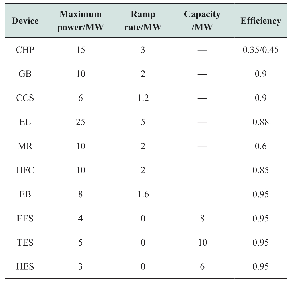
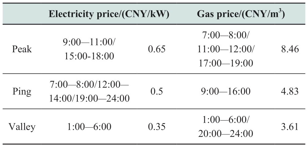
To illustrate the accuracy and effectiveness of the model proposed in this paper, the simulation data include the measured data of a certain location in the north. The sampling period is 1 h, and the total number of samples is 2400. The forecast error of the electrical, thermal, and gas loads is set to 10%. Using the 2.3 section method,1000 load-energy consumption scenarios are generated.Finally, 10 typical load-demand scenarios are obtained by reduction. The self-elastic coefficients of the electrical and gas loads are −0.1 and −0.2, respectively, and the cross-elastic coefficient is 0.03 [33, 34]. The proportions of transferable and reducible loads in the electrical and gas loads are 20% and 10% of the total load, respectively.The carbon transaction cost is 80 CNY/t. The energy price and equipment-related parameters are listed in Table A1(Appendix) and Table 1, respectively.

Table 1 Device operating parameters

4.2 Comparative analysis of different estimation methods

To verify the effectiveness of the IRKDE proposed in this paper, the relative error percentage of wind power and PV output prediction are set to ± 20% and ± 15%,respectively. The historical wind and light prediction error data obtained by sampling are fitted using the KDE,Variable kernel density estimation (VKDE), RKDE, and IRKDE methods. To ensure and highlight the comparison of the fitting effects of the different estimation methods,the selected fixed smoothing parameter is 0.02. The fitting probability density results of the different estimation methods are shown in Figs. 3 and 4.

As shown in Fig. 3, the KDE and VKDE are used to fit the probability density of wind power and PV output prediction error information. The KDE method is better than the VKDE method in fitting both sides of the information distribution. In contrast, the VKDE method is better than the KDE method in fitting the spike area (i.e., central region) of the information distribution. The KDE method uses fixed smoothing parameters for fitting that cannot be used for the statistical information intervals of frequency differences; it cannot be flexibly adjusted. In contrast,the VKDE method uses variable smoothing parameters that can be flexibly adjusted according to the distribution characteristics of observations. Thus, VKDE can achieve better fitting than KDE in the spike region. The RKDE and IRKDE methods are used to fit wind power and PV output prediction errors, as shown in Fig. 4. The IRKDE method is more accurate than RKDE in fitting wind boundary extremes and PV output error intervals. Its fitting accuracy in the spike region is more accurate than that of the RKDE.Hence, the IRKDE method’s overall fitting of the wind and PV historical output prediction error data is better than that of the RKDE method. The RKDE method uses fixed smoothing parameters, and the overall fitting effect is still affected by the interval boundary observations. In contrast,the IRKDE method appropriately adjusts the smoothing parameters assigned to each observation of the sample data according to the distribution information. The overall sum of errors for the entire sample is minimized because the fixed parameters and data outliers are simultaneously processed. Local intervals with high fitting errors are corrected by adjustable smoothing coefficients, replacing the traditional fixed smoothing parameters. Therefore, the method used in this study increases the fitting accuracy of the overall probability distribution. By assigning adaptive smoothing parameters to each sample value, the model error can be effectively reduced, thereby improving the overall goodness of fit. The difference between IRKDE and KDE is that the former can improve the effects of interval outliers or extreme values. Thus, the IRKDE model is more suitable for practical engineering.

Fig. 3 Fitting results of probability density distribution of KDE and VKDE

Fig. 4 Fitting results of probability density distribution of RKDE and IRKDE

4.3 Optimization of scheduling results

The influence of wind and light uncertainties determined by the four estimation methods on the optimal scheduling of the system can be verified as follows. Assume that the confidence level of the scenery output is 0.95 when the deviation of the prediction of the wind and PV outputs is maximum. Then, at this level, establish the optimal scheduling model using the four methods. The system operation costs are summarized in Table 2.

Table 2 Comparison of system operating costs of different estimation methods

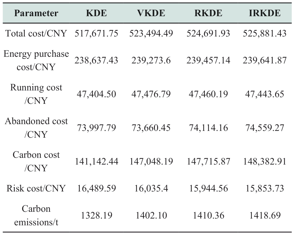
The cost comparison indicates that the total system cost resulting from the use of the style="font-size: 1em; text-align: justify; text-indent: 2em; line-height: 1.8em; margin: 0.5em 0em;">The results of the proposed robust stochastic optimization using the IRKDE data estimation method to drive the uncertainty sets are shown below.

Consider the scheduling of electric energy as an example; the power optimization results are shown in Fig. 5.The output of wind power at night is at its peak, and the electric load is in the valley period. Hence, wind power is not completely consumed from 01:00 to 07:00 and from 22:00 to 24:00; however, it is timely consumed from 8:00 to 16:00. The PV power output is high although the Integrated demand response (IDR) strategy is considered to increase the electric load, and EB converts electric energy into heat energy. A small extent of wind and PV power abandonment exists, resulting in low energy utilization and rising operating costs. For scenario 1, the addition of a hydrogen energy system is considered. Thus, the flexibility of hydrogen energy utilization is fully utilized, and the coupling between electricity, heat, and gas is strengthened.Excess electric energy can be converted into hydrogen through the EL equipment during the surplus period of wind power output. The HFC and MR supply electricity,heat, and gas loads, and the HES device transfers energy,effectively increasing the utilization rate of wind power and the flexibility of the system. Owing to the improvement in energy efficiency and reduction in carbon emissions, the total cost of the IES decreases.

Fig. 5 Power optimization scheduling results

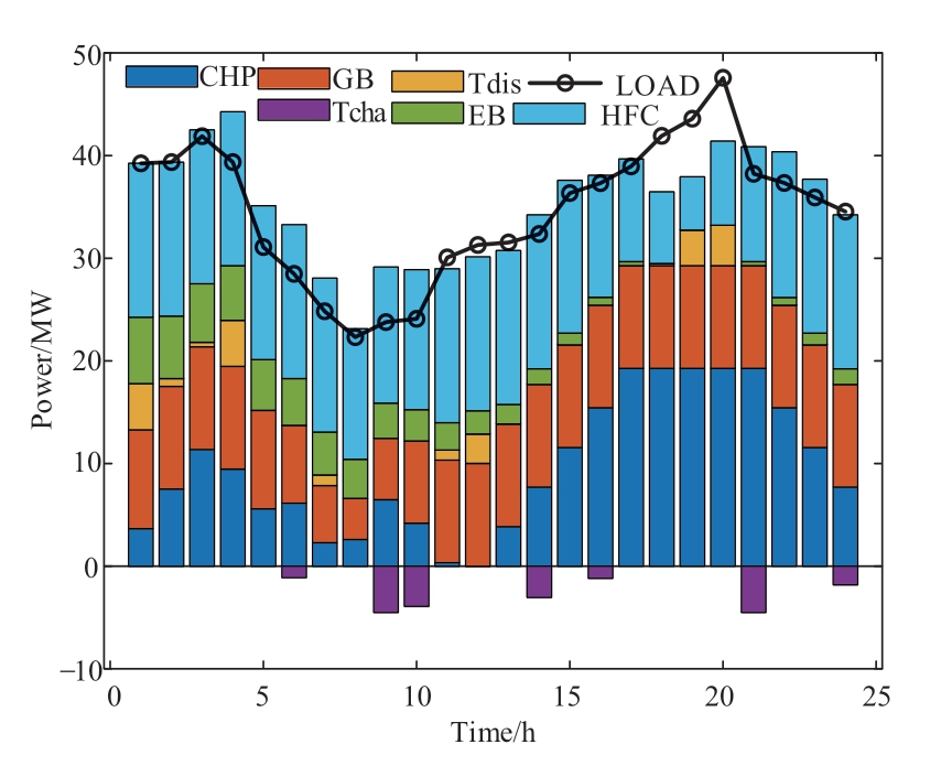
Fig. 6 Thermal power optimization scheduling results

For the scheduling results, the IEPU first inputs surplus wind power into the EL to produce hydrogen and then absorbs the remaining wind power. Part of the hydrogen produced by the EL is then transported to the HFC to provide electricity and heat. The other part is sent to the MR synthetic natural gas or stored in the HES. Different from the transportation of hydrogen energy through the MR synthesized natural gas to the GB or CHP, the production of heat and electricity from hydrogen energy through the HFC to the user reduces the consumption of an energy cascade. To improve the efficiency of energy utilization,the IEPU prioritizes the transportation of hydrogen energy to the HFC for thermoelectric production. Then, it sends the remaining part of the energy to the MR or HES. The optimal scheduling results of hydrogen power are shown in Fig. 8. The time-of-use electricity price (time period: 9:00–11:00) is higher than the time-of-use gas price (time period:15:00–18:00); hence, releasing the hydrogen energy for the HFC is appropriate. In the period of low electricity price,hydrogen is mainly produced and stored in the EL. The MR synthesizes methane to supply a gas load, whereas the HFC burns H2 to produce electricity and heat. This reduces the dependence of the gas load on natural gas and realizes the full utilization of H2.

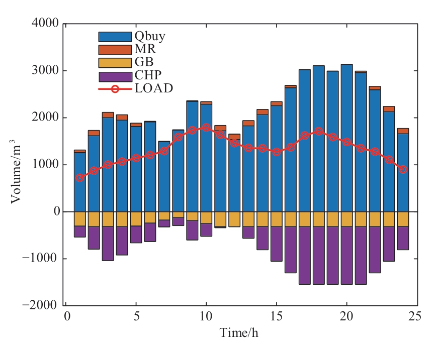
Fig. 7 Gas power optimization scheduling results

As shown Fig. B1 (Appendix), after the demand response, the peak-valley difference of electrical load use decreases by 4% compared with the difference before the demand response. The peak-valley difference of the gas load also decreases by 2.4%. Moreover, the load fluctuation is significantly stabilized. First, because of the impact of the price response on the energy consumption habits of users, the load of users shifts downward and upward during the peak and valley periods of the price, respectively.During the normal period, the load is adjusted according to the load changes during the peak and valley periods.The effectiveness of the price-based demand response for optimizing the electricity and gas loads is verified. Second,because the power storage and heating equipment can act as an energy supplier or a consumer according to the system requirements, peak shaving and valley filling are affected.Additionally, thermal energy users are ensured that the heat demand is flexibly adjusted according to the energy operation of the system without affecting thermal comfort.Further, heat is transferred from the peak period to the trough period, and the energy supply pressure of the sourceside equipment is reduced. This shows that by optimizing the operation, the load energy load curve can be effectively smoothed, providing a guarantee for improving economy,environmental protection, and energy efficiency of the system operation.

Fig. 8 Hydrogen power optimal scheduling results

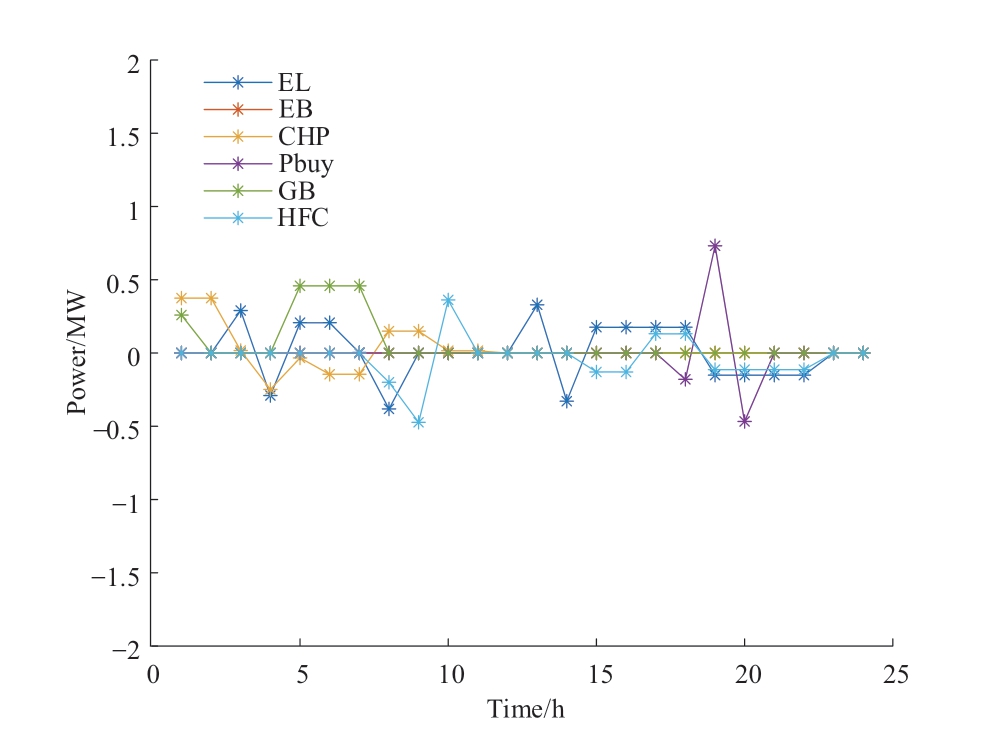
Fig. 9 Difference in optimal output values between robust stochastic model and robust model when σ = 0.9

Fig. 10 Difference in optimal output values between robust stochastic model and robust model when σ = 1.1

The influence of different load scenarios on the scheduling results is analyzed. Multiple predicted values of the load demand under different load scenarios are defined.The difference in equipment energy consumptions between robust optimization and robust stochastic optimization when σ = 0.9 and σ = 1.1 is shown in Figs. 9 and 10, respectively.The power difference fluctuation of the EB is low under different load scenarios, whereas the power difference of the EL, GB, HFC, CHP, and tie lines are higher. This is because the system considers the problem of system carbon emissions and preferentially selects the HB to satisfy the heat load. Because the time-of-use electricity and gas prices are considered during high load fluctuations, the nighttime electricity and gas prices are in the trough period. The load fluctuation is mainly stabilized by the EL, GB, HFC, and CHP. During daytime or ordinary times when the energy price is at its peak, the EL is mainly used for converting electricity to hydrogen. In contrast, the HFC is used for cogeneration, and the MR is used for converting hydrogen to natural gas to reduce the dependence on superior natural gas. Finally, when the system power balance is difficult to maintain, the tie line bears the system power shortage, and the power difference of the tie line changes significantly.Therefore, under random load fluctuations, the robust stochastic optimization scheduling method can flexibly adjust the equipment according to the market price and equipment characteristics.

4.4 Influence of uncertainty parameters on system operation

To verify that the robust optimization method proposed in this study can flexibly adjust to the conservativeness of the scheduling scheme, several sets of uncertainty regulation parameters are selected for simulation comparison; results are summarized in Table 3. In the table, note that the wind and PV power uncertainty regulation parameters are Γ wt =12 and Γ pv =6, respectively. This indicates that the PV outputs are considered as the maximum and minimum values of the prediction interval for 12 (at most) and 6 time periods, respectively, during the scheduling optimization process. The rest of the time periods are equal to the predicted value.

Table 3 indicates that the uncertainty regulation parameter is 0. This is equivalent to deterministic optimization without considering the uncertainty of the wind and PV power forecast errors. The system operation cost increases with the uncertainty regulation parameter. Hence, the greatest uncertainty confronting the system is considered when formulating the dispatching plan. The higher the value of Γ, the more the number of time periods when the wind power and PV output are considered the maximum value of the forecast interval. The greater the conservativeness of the solution, the higher the required system investment;consequently, the corresponding operating cost is higher.By modifying the uncertainty regulation parameters, the conservativeness of the microgrid optimization scheme can be flexibly adjusted. This benefits the IES dispatcher in terms of reasonably choosing between operating cost and risk.

Table 3 Comparison of optimization results of different uncertainty parameters

5 Conclusions

In this study, a style="font-size: 1em; text-align: justify; text-indent: 2em; line-height: 1.8em; margin: 0.5em 0em;">1) The proposed method uses the IRKDE method to establish the probability distribution function of the renewable energy prediction error. The proposed method reduces the subjective selection of smoothing parameters of the traditional RKDE. It effectively considers the smoothing effect and accuracy of model fitting. Moreover, it adapts to statistical information, and avoids overfitting.

2) The constructed distributed robust optimization method is a combination of stochastic optimization and robust optimization. It can make full use of the statistical information of historical output data and the random scenario of uncertain load energy consumption, ensure the economy of system operation and improve the robustness of the system, and better realize the coordinated emission reduction of source and load.

3) Considering the two-stage process of P2G and the introduction of hydrogen storage device and hydrogen fuel cell to make full use of the advantages of hydrogen energy and comprehensive demand response, it can effectively reduce the carbon emissions of the system, reduce the energy abandonment rate of renewable energy, and improve the flexibility of system operation.

In the future, we can consider improving the RKDE method or using other statistical tools to obtain more accurate data distribution information. In this paper, the source-load uncertainty of the integrated energy system with hydrogen energy utilization is established for robust optimal scheduling. It is considered that the energy efficiency of the equipment model in this paper is unchanged, but the equipment is dynamic in actual operation. In the future, the robust optimal scheduling of equipment dynamic energy efficiency under source-load uncertainty environment can be considered more detailed and practical.

Appendix A

The general mathematical form of the mixed integer linear programming (MILP) problem with uncertain quantities can be formulated as follows:

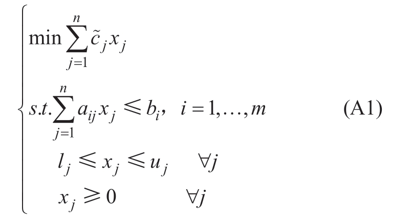
Here, if  is a variable with uncertainty, then equation(A1) is the MILP problem with uncertainty. To facilitate the description, let take the value in [ c j,c j+d j], where cj is the minimum value of the uncertainty  (let it be the standard value) and dj is the maximum deviation of the uncertainty  with respect to the standard value cj.

Model (A1) is transformed into:

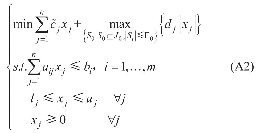
Make:

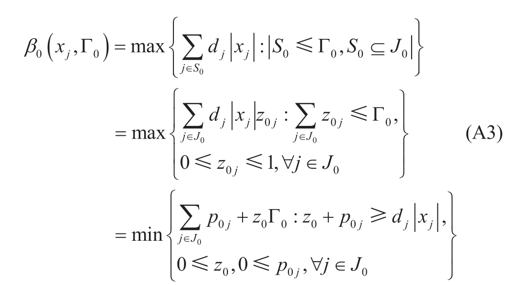
Substitution yields the final robust optimization form as

Table A1 Energy price

Appendix B

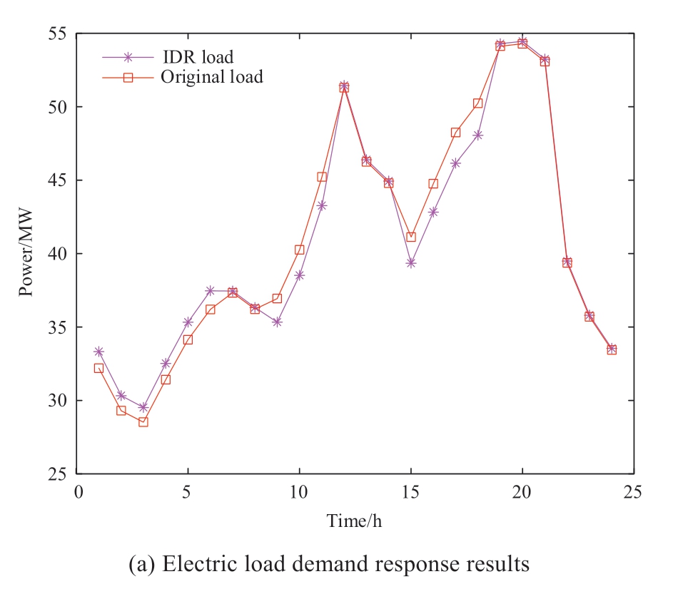
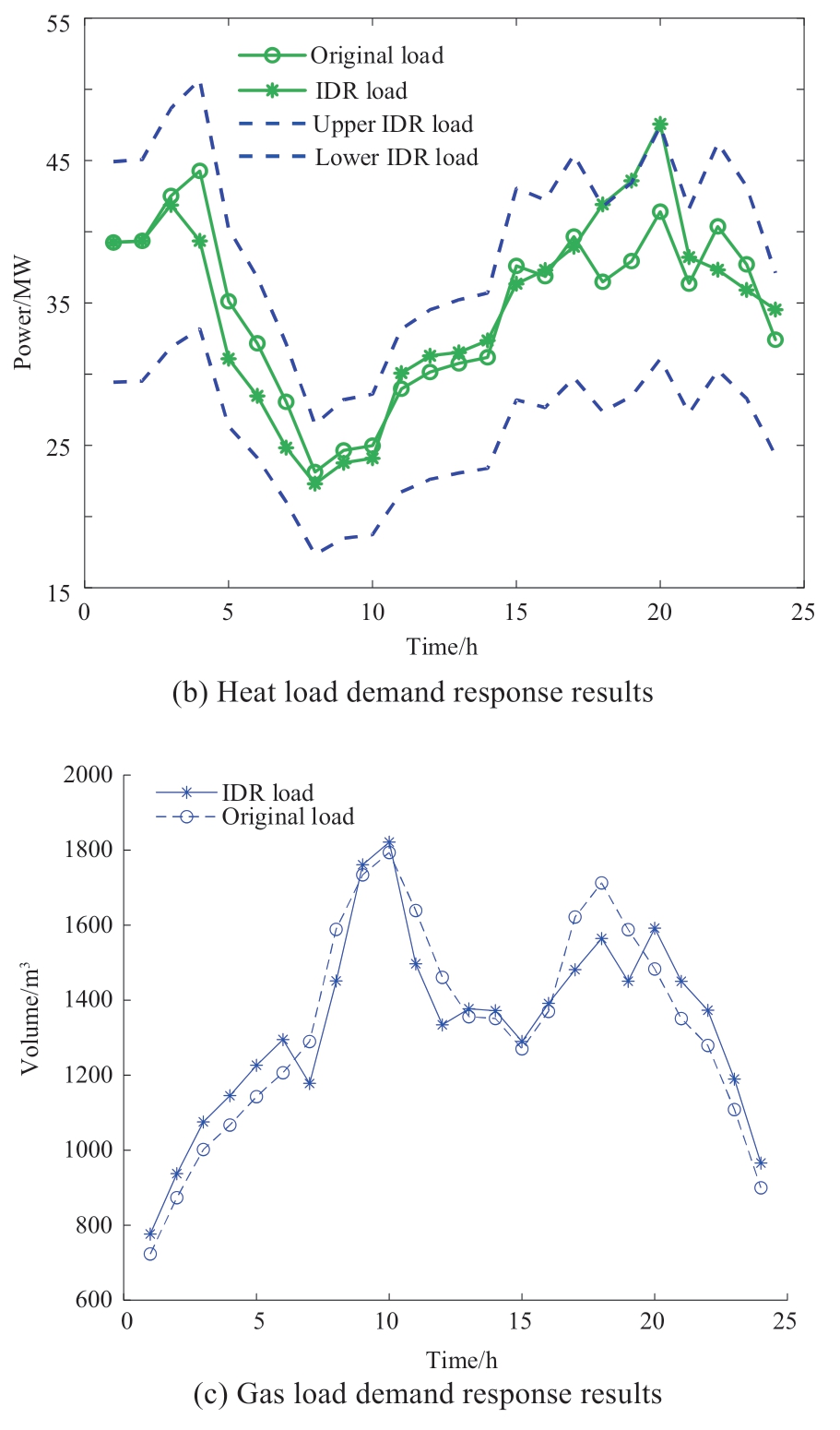
Fig. B1 IDR scheduling results

Acknowledgements

This work was supported by the National Key Research and Development Project of China (2018YFE0122200).

Declaration of Competing Interest

We declare that we have no conflict of interest.

References

[1] Sanja P, Lidija Č, Mariano M, et al. (2021) Sustainable renewable energy supply networks optimization-The gradual transition to a renewable energy system within the European Union by 2050.Renewable and Sustainable Energy Reviews, 146: 111186

[2] Li Y, Bu F, Gao J, et al. (2022) Optimal dispatch of low-carbon integrated energy system considering nuclear heating and carbon trading. Journal of Cleaner Production, 378: 134540

[3] Lv C, Yu H, Li P, et al. (2019) Model predictive control based robust scheduling of community integrated energy system with operational flexibility. Applied Energy, 243: 250-265

[4] Abu-Rayash A, Dincer I (2020) Development of an integrated energy system for smart communities. Energy, 202: 117683

[5] Zhao N, You F (2021) New York State’s 100% renewable electricity transition planning under uncertainty using a datadriven multistage adaptive robust optimization approach with machine-learning. Advances in Applied Energy, 2: 100019

[6] David P, Zhang X, Christian B, et al. (2017) An integrated techno-economic and life cycle environmental assessment of power-to-gas systems. Applied Energy, 193: 440-454

[7] Yin L, Tao M (2023) Balanced broad learning prediction model for carbon emissions of integrated energy systems considering distributed ground source heat pump heat storage systems and carbon capture & storage. Applied Energy, 329: 120269

[8] Zhou Q, Zhao Y, Zhang L (2021) Integrated energy production unit: An innovative concept and design for energy transition toward low-carbon development. CSEE Journal of Power and Energy Systems, 7(6): 1133-1139

[9] Ma Y, Wang H, Hong F, et al. (2021) Modeling and optimization of combined heat and power with power-to-gas and carbon capture system in integrated energy system. Energy, 236: 121392

[10] Wang J, Mao J, Hao R, et al. (2022) Multi-energy coupling analysis and optimal scheduling of regional integrated energy system. Energy, 254: 124482

[11] He J, Wu Y, Yong X, et al. (2022) Bi-level optimization of a near-zero-emission integrated energy system considering electricity-hydrogen-gas nexus: A two-stage framework aiming at economic and environmental benefits. Energy Conversion and Management, 274: 116434

[12] Wu Q, Li C (2023) Modeling and operation optimization of hydrogen-based integrated energy system with refined powerto-gas and carbon-capture-storage technologies under carbon trading. Energy, 270: 126832

[13] Gu Z, Pan G, Gu W (2022) Portfolio of wind-photovoltaicloads toward green hydrogen development. Proceeding of 2022 IEEE 5th International Electrical and Energy Conference(CIEEC), Nangjing, China, pp. 4988-4993, doi: 10.1109/CIEEC54735.2022.9846412

[14] Pan C, Jin T (2023) Multi-objective and two-stage optimization study of integrated energy systems considering P2G and integrated demand responses. Energy, 270: 126846

[15] Yang P, Jiang H, Liu C, et al. (2023) Coordinated optimization scheduling operation of integrated energy system considering demand response and carbon trading mechanism. International Journal of Electrical Power & Energy Systems, 147: 108902

[16] Moghadam T A, Soheyli F, Sanei S, et al. (2022) Bi-level optimization of the integrated energy systems in the deregulated energy markets considering the prediction of uncertain parameters and price-based demand response program. Energy Science &Engineering. 10: 2772-2793

[17] Gu H, Li Y, Yu J, et al. (2020) Bi-level optimal low-carbon economic dispatch for an industrial park with consideration of multi-energy price incentives. Applied Energy, 262: 114276

[18] Li J, Wang C, Li G, et al. (2021) Optimal scheduling of integrated demand response-enabled integrated energy systems with uncertain renewable generations: A Stackelberg game approach.Energy Conversion and Management, 235: 113996

[19] Cao Z, Wang J, Zhao Q, et al. (2021) Decarbonization scheduling strategy optimization for electricity-gas system considering electric vehicles and refined operation model of power-to-gas.IEEE Access, 9: 5716-5733

[20] Chen M, Lu H, Chang X, et al. (2023) An optimization on an integrated energy system of combined heat and power, carbon capture system and power to gas by considering flexible load.Energy, 273: 127203

[21] Wang Y, Yang Y, Fe H, et al. (2022) Wasserstein and multivariate linear affine based distributionally robust optimization for CCHP-P2G scheduling considering multiple uncertainties. Applied Energy, 306: 118034

[22] Sahar R, Wang Z, Ju P (2022) Overview and applications of Robust optimization in the avant-garde energy grid infrastructure:A systematic review, Applied Energy, 319: 119140

[23] Ning C, You F (2019) name="ref24" style="font-size: 1em; text-align: justify; text-indent: 2em; line-height: 1.8em; margin: 0.5em 0em;">[24] Fang F, Yu S, Xin X (2022) name="ref25" style="font-size: 1em; text-align: justify; text-indent: 2em; line-height: 1.8em; margin: 0.5em 0em;">[25] Baharvandi A, Aghaei J, Niknam T, et al. (2018) Bundled generation and transmission planning under demand and wind generation uncertainty based on a combination of robust and stochastic optimization. IEEE Transactions on Sustainable Energy, 9(3): 1477-1486

[26] Xin P, Liu Y, Yang N, et al. (2020) Probability distribution of wind power volatility based on the moving average method and improved nonparametric kernel density estimation. Global Energy Interconnection, 3(3): 247-258

[27] Liu G, Zhu Y, Huang Z (2020) Dynamic economic dispatch with wind power penetration based on non-parametric kernel density estimation. Electric Power Components and Systems, 48: 333-352

[28] Wei H, Hou W, Zhu R (2019) A name="ref29" style="font-size: 1em; text-align: justify; text-indent: 2em; line-height: 1.8em; margin: 0.5em 0em;">[29] JooSeuk K, Clayton D S (2012) Robust kernel density estimation,Journal of Machine Learning Research, 13: 2529-2565

[30] Zhang Z, Zhang Y (2014) Variable kernel density estimation based robust regression and its applications. Neurocomputing,134: 30-37

[31] Wang Y, Wang Y, Huang Y, et al. (2019) Optimal scheduling of the regional integrated energy system considering economy and environment. IEEE Transactions on Sustainable Energy, 10(4):1939-1949

[32] Zhang R, Jiang T, Li G, et al. (2018) Day-ahead scheduling of multi-carrier energy systems with multi-type energy storages and wind power. CSEE Journal of Power and Energy Systems, 4(3):283-292

[33] Chen Y, Ma Y, Zheng G, et al. (2022) Coordinated planning of multi-CHP units considering demand response. Power grid technology, 46(10): 3821-3832

[34] Wang L, Xu J, Li S, et al. (2022) Low-carbon economic dispatch of integrated energy system considering electricity-gas-heat demand response and stepwise carbon trading. Smart Power,50(9): 45-52

Received: 8 April 2023/ Accepted: 5 July 2023/ Published: 25 August 2023

Dingyue Huang

huang_dingyue@163.com

Jinling Lu

lujinling@126.com

Hui Ren

hren@ncepu.edu.cn

2096-5117/© 2023 Global Energy Interconnection Development and Cooperation Organization. Production and hosting by Elsevier B.V. on behalf of KeAi Communications Co., Ltd. This is an open access article under the CC BY-NC-ND license (http: //creativecommons.org/licenses/by-nc-nd/4.0/ ).

Biographies

Jinling Lu received bachelor’s degree at North China Electric Power University in 1993,Baoding; received master’s degree at North China Electric Power University in 1996,Baoding; received PhD at North China Electric Power University in 2009, Baoding. Now, she is working as an associate professor in North China Electric Power University, Baoding.

Dingyue Huang received the bachelor’s degree from Northeast Electric Power University, Jilin, 2021. She is currently pursuing master’s degree in North China Electric Power University, Baoding. Her main research fields are Power system operation,analysis and control.

Hui Ren received bachelor’s degree at North China Electric Power University in 1994,Baoding; received master’s degree at North China Electric Power University in 1997,Baoding; received PhD at North China Electric Power University in 2009, Baoding. Now,she is working as a professor in North China Electric Power University, Baoding.

(Editor Yajun Zou)