0 Introduction

With the rapid development of artificial intelligence and big data technology,data have become a primary factor of production in the modern era.Both the data sources and types are becoming increasingly diversified and complicated,which makes the integration of multi-source heterogeneous data an inevitable trend.Aiming to achieve intellectualization of the power grid,more monitoring,control,and transmission devices are integrated,as well as access to renewable energy sources and electricity terminals.The storage,processing,and efficient utilization of multi-source heterogeneous data generated by the grid,particularly when the data are distributed across different physical environments,present considerable challenges for the development of new power systems.They are also key issues in achieving situational awareness,diagnosis,and decision making for the smart grid.

To solve the aforementioned problems,some existing studies have utilized big data techniques to store and process data[1].For example,frameworks based on Spark[2]and GraphX[3]have been proposed to process massive amounts of data in power grids.However,when used for memory-based power grid computation,these methods based on big data architecture require frequent data import and export operations,which results in significant overhead.Meanwhile,for analysis and mining scenarios depending on large-scale multi-source heterogeneous data fusion in power grids,traditional relational data models seem overwhelming to satisfy these complex tasks.As an increasingly mature non-relational data model,graph database is highly suitable for handling the association relationship between entities with heterogeneous information.Real world scenarios with typical graph patterns,such as power grids,social networks,traffic networks,etc.have a natural advantage to use graph databases to store and analyze data.Therefore,some researchers have adopted graph databases for data modeling and data management in power systems.For instance,previous studies have used the Neo4j graph database to store transmission grid data[4]and achieve modeling grid system and analyzing topology[5].Such studies based on graph databases have primarily focused on the representation and storage of power systems,whereas few studies have considered combining graph databases with power grid computation,failing to fully utilize the distributed parallel computing potential of graph databases.

In some graph applications,such as recommendation systems[6],road traffic[7],and biomedicine[8],conventional graph algorithms are principally applied,including shortest path algorithms,community detection algorithms,etc.In addition to these conventional algorithms,some specific graph schema scenarios,such as power grid computations require a large number of matrix computations.However,there is little existing work related to matrix computation based directly on graph modelling,and the current mainstream graph database products,which mostly focus on storage and query,lack native support for matrix computations.

Considering the wide application of matrix computations in power systems and the inherent correlation between graph and matrix models,this study investigates a general graph description method for matrix computation based on a graph database.The analysis aims to simplify and accelerate the computation process.Based on the proposed method,some typical power grid computational tasks are implemented in the graph database.In summary,the contributions in this study are outlined as follows.

1)A general graph description approach for matrix computation is designed with a variety of typical matrix operations(matrix multiplication,matrix decomposition etc.)based on the native graph structure.

2)Comparative experiments on the graph description method verify the superiority of the proposed method to the conventional traversal method and demonstrates its higher parallelizability.Moreover,the factors that affect parallel computation are investigated.

3)Based on the proposed graph description method,a solution is developed in the graph database for typical grid applications of power flow calculation and N-1 contingency computation,and the corresponding experimental results show the effectiveness.

The remainder of this paper is organized as follows.The next section briefly reviews the power calculation and graph databases.Section 2 details the principle and implementation of the graph description method proposed in this paper.Section 3 presents the results of comparative application experiments for typical matrix calculations.Based on the proposed method and the graph database,Section 4 verifies the effectiveness of parallel computing,and Section 5 outlines the power flow calculation.Finally,the last section concludes this paper.

1 Related work

1.1 Scientific computing for power

For power flow calculations,steady-state and grid safety analysis,the matrix operation is one of the most fundamental and core problems.To this end,a series of studies have been conducted to speed up computation and improve the real-time response.Xie et al.[9]utilized the Gaussian elimination with static pivoting(GESP)algorithm to solve Newton’s power flow equation and developed the parallel process on a distributed platform.Based on a heterogeneous CPU-GPU architecture,Wei et al.[10]combined the inexact Newton’s method with a two-phase bi-conjugate gradient stabilized method,which significantly improved the efficiency compared to the conventional Newton-Raphson computation.Similarly,Yang et al.[11]performed calculations on compute unified device architecture(CUDA).Zhang et al.[12]used an implicit Cholesky decomposition algorithm to solve the Levenberg-Marquardt iteration,which reduced the redundant computations.Liu et al.[13]studied parallel computation over a GPU and proposed a 3-tier parallel architecture for multi-case and individual power flow computation.The above methods aimed at improving the computational efficiency using hardware platforms;however,they have two limitations.First,none of them considered the management and modeling of multi-source heterogeneous data,which would limit their availability in new power systems.Second,similar to[2,3],there exists massive data I/O overhead that cannot be ignored.

From another perspective,the acceleration of matrix calculation is also an option.Blalock et al.[14]designed a learning-based algorithm for approximating matrix multiplication.Similarly,Fawzi et al.[15]introduced the first AI system AlphaTensor to provide efficient and correct algorithms for basic matrix multiplication tasks.Based on the FPGA framework,Zhou et al.[16]converted the matrix decomposition algorithm based on random gradient descent into a bipartite graph processing problem,whose performance was improved by more than an order of magnitude,compared to the optimized accelerator based on GPU.Nevertheless,the above studies cannot be applied directly to relational and graph databases.

Similar to the basis of our work,there are solutions to grid computing based on the graph model.Dai et al.[17]developed grid topology based on GraphSQL.They utilized the graph traversal algorithms to design a more efficient method for grid outage regions analysis.Jiang et al.[18]investigated a preferable approach for power supply reliability analysis on distribution network using highspeed bi-directional breadth-first search of Neo4j graph schema.Zhao et al.[19]solved “N-1” contingency analysis by incorporating the preconditioning conjugate gradient algorithm to the native bulk synchronous parallel feature of graph database,whose performance is superior to that of the traditional calculation method.The aforementioned studies took advantage of graph databases in both the graph computation and parallel computation for efficiency improvement compared to traditional methods and relational database-based methods.However,none of them consider how to use graph databases to optimize the matrix calculation involved in grid computation.

1.2 Graph database

A native graph database represents the sets of entities and associative relationships between them in terms of vertices and edges,respectively.Attributes of arbitrary data types can be attached to both vertices and edges in the form of key-value data.The logical model,query model,and underlying storage of the native graph database are all in the form of graph without third-party storage components,which provides excellent performance in query and management for graph applications with multi-hop query.In contrast,a relational database organizes relationships between entities using extra tables along with multiple paradigm constraints,which results in data redundancy and expensive or even infeasible execution cost for multi-hop queries.Liu et al.[20]illustrated the differences between graph databases and relational databases using an electric power system.The authors compared the performance gap for all the regular operations and highlighted the significant advantages of graph databases over relational ones.Based on the same datasets,Cheng et al.[21]further verified that graph databases exhibit superior performance for multi-table joins,pattern matching,path recognition,etc.

1.3 Graph applications

For real-world scenarios with strong correlation,it is more direct and appropriate to use a graph model to comprehensively explore the hidden value from the data.In[22],the traffic network was modeled as a directed graph with road segments as edges and intersections between segments as vertices,where the travel time of a path can be estimated using the graph.Yin et al.[23]modeled a network of monitoring sensors as an undirected graph,in which the sensors were represented as vertices and the accessibility between sensors as directed edges.The authors used the graph for predicting traffic flow.Wang et al.[24]developed a social network with vertices and edges to represent users and the corresponding social relations between them,e.g.,mentioning,following,and being followed.Based on the social graph,the resident locations of users can be predicted.In[25],components in the power system topology were directly mapped into a distribution network graph database.Different labels were allocated to various types of devices.Utilizing graph path algorithms,they implemented reliability analysis over the distribution network graph.Obviously,the graph pattern can be used in various scenarios for different tasks,modeling sundry relationships,and mining complex objectives.

2 Graph description of matrix calculation

2.1 Applications of matrix calculation

Matrix operations occupy a crucial position in various fields,such as image processing,operation planning,power grid computation,machine learning,etc.In image processing,a picture is often represented as a matrix that can be decomposed,transformed,and used to extract eigenvalues.In the field of operation planning,decision variables are modeled into a matrix to handle optimization problems.In power systems,power flow calculation plays a crucial role in all phases of grid planning,operation,and fault detection.Existing mainstream approaches,such as Gauss-Seidel iteration,Newton-Raphson method,and PQ decomposition method,require derivative matrices and Jacobi matrices,etc.For machine learning,various optimization computations gradually evolve into matrix problems,whose core often lies in the matrix operations for solving non-simultaneous linear systems of equations.Moreover,matrix decomposition is a regular strategy to reduce cost to accelerate the evaluation over large scale data.Hence,matrix calculation has a pivotal role in many disciplines.

2.2 Correspondence between graph and matrix

Besides the topological representation of a graph,there are various data structures,such as adjacency matrix,adjacency linked table,cross-linked table,etc.Owing to the intuition and computational convenience of the adjacency matrix,the adjacency is commonly used for graph calculation.Specifically,we denote a graph as G=(V,E,A),where V and Erepresent the sets of vertices and edges,respectively.N indicates the cardinality of V.Each element aij in the adjacency matrix  indicates whether vertices i and j are connected,and we refer toas the corresponding edge for consistency.Let aij=0 if there is no edge between i and j,otherwise it represents the weight on edge pointing from i to j.If G is an undirected graph,A represents a symmetric matrix.The non-zero elements in the i-th row(resp. j-th column)of matrix A denotes the existence of edges pointing from i to the other vertices(resp.from the other vertices to j).Accordingly,the neighbors of each vertex can be easily derived.Figure 1 illustrates the correspondence between the matrix and the graph.For each non-zero non-diagonal element in the matrix,there is an edge in the graph corresponding to it.For non-zero diagonal elements,they are vertices pointing to themselves,which is referred to as a self-edge in this paper,e.g.,edge in Fig.1.The values of non-zero elements represent the weights of edges.

Fig.1 Correspondence between matrix and graph:(a)5×5 square matrix,where 。denotes the zero element;(b)the corresponding graph

2.3 Graph description of typical matrix operations

As discussed above,the structure of the graph visually depicts the correlation between various entities,and thus an increasing number of storage and analysis tasks with complex relations or multi-source heterogeneous data are implemented over graph databases.Many analytical tasks rely on matrix calculation,and almost all the existing graph database products lack native support functions or API interfaces for matrix calculation.As a result,many graph computations cannot be completed in graph databases.This requires querying the data from the database and storing the results back in the database after calculations by external programs with extra data transfer overhead,such that the graph database is only a data storage tool that fails to fully realize its analytical and computational capabilities,limiting the usage scope.To this end,we propose a matrix computation method based on graph description,so that the graph database can have the capability of matrix computation and reduce the data transfer overhead by running matrix computation tasks inside the database.

This subsection elaborates on the graph description implementation process of two typical matrix operations,i.e.,matrix multiplication and matrix decomposition.To better discuss the calculation process,we use two other designations,namely neighbor-edge and mutual-edge,besides self-edge.The former corresponds to an edge that points from one vertex to another,as edge shown in Fig.1.Given a specific vertex i,the latter designation indicates the edge that connects two neighbor vertices of i.For example,edge in Fig.1 is a mutual-edge of vertex 3,which connects its neighbor vertices 2 and 5.

2.3.1 Graph description of matrix multiplication

The matrices involved in matrix multiplication are not forced to be square,so for matrices A∈ℝm×n and B∈ℝn×l,we have AB=C∈ℝm×l.Adjacency matrices are generally square.Hence,when we transform and describe a matrix using a graph,the number of vertices of the graph should be consistent with the largest row or column dimension of the matrix.In this study,we use the notation G(A)to indicate the graph description of matrix A.Specifically,if n≥m(resp.n≤m),the number of vertices in G(A)equals n(resp.m)following the transformation.The number of edges is the same as the number of non-zero elements in the nondiagonal elements.The vertices numbered greater than m(resp.n)in G(A)have no edges pointing to them and their indegrees(resp. outdegrees)are set to zero.As illustrated in Fig.2(a),the dimension of the matrix is 5 × 3,which means that there are five vertices in the transformed graph,as shown in Fig.2(b),where the vertices 4 and 5 have no incoming edges.

Fig.2 Transformation on non-square matrix:(a)matrix with unequal row and column dimensions;(b)the graph description of the matrix in(a)

According to the definition of matrix multiplication,each element cpq in matrix C can be derived from(1),where api and biq represent the elements of matrices A and B,respectively.

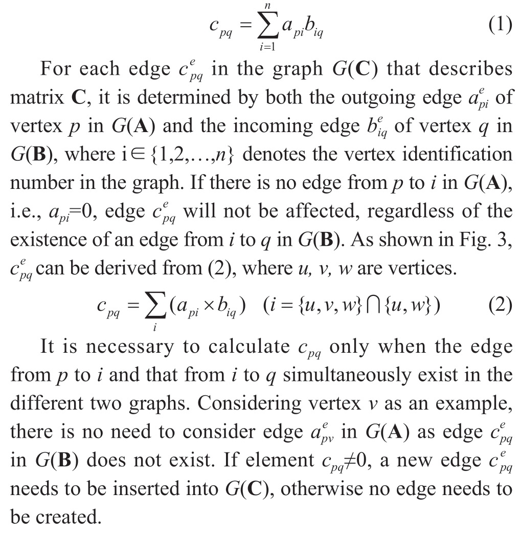
Fig.3 The parts of the two graphs involved for the outgoing edges of p in G(A);(b)the incoming edges of q in G(B)

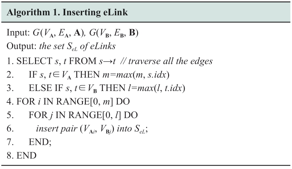
Hence,we can add m× l new edges to G(C)to quickly find the vertices in both G(A)and G(B)that correspond to each element in C.These new edges are connected by each vertex in G(A)with non-zero outdegree to every vertex in G(B)with non-zero indegree,respectively.We denote such edges as eLinks,each of which is used to represent the correlation between an edge located in G(C)and its two endpoint vertices that are in G(A)and G(B),respectively.In the graph description method,the eLinks are created without storing any property value and used to assist the computation process of matrix multiplication,whereas they do not participate in the calculation themselves.Each eLink needs to be created before executing the matrix multiplication,and it can either be imported into the database along with G(A)and G(B),or created by inserting new edges when querying G(A)and G(B).The insertion process of eLinks over G(A)and G(B)is detailed in Algorithm 1.To distinguish the vertex sets and edge sets of different graphs,we use the corresponding matrix names as set subscripts to identify them,e.g.,VA and EB are the vertex set and edge set of matrix A and B,respectively.

In Algorithm 1,we first initialize the values of m and l of G(A)and G(B),respectively(lines 1-3).In line 1,the expression s→tindicates a graph schema that query all edges and their two endpoints s and t.The property idx indicates the index number of a vertex(lines 2-3).The insertion of each eLink into the graph database is conducted in line 6,whose source and target vertices are the i-th vertex in VA and the j-th one in VB.For ease of exposition,all the eLinks stored in database are regarded as organized in the set SeL of eLinks.

On inserting the eLinks into the graph database,the matrix calculation process based on the graph description method is outlined in Algorithm 2.Both the outgoing and incoming edges are represented by a key-value edge pair of the form(idx,val),where val indicates the weight on the edge.For an outgoing edge,the variable idx in the edge pair corresponds to the index of target vertex t,and should be stored into the outgoing edge set Out of the corresponding source vertex s.Similarly,for an incoming edge,idxindicates the index of source vertex s,and needs to be stored in the incoming edge set In of the corresponding target vertex t.In other words,each source vertex has a set of outgoing vertices with the edge weights(Out),and vice versa for target vertices.

First,we find the outdegree neighbors of each vertex in G(A)(i.e.,the vertex has outgoing edges pointing to the neighbors)and indegree neighbors in G(B)(i.e.,the vertex is the target vertex of its neighbors).The neighbors being found are stored as edge pairs into set Out or In,based on whether they are target or source vertices(lines 1-4).The query expression s-(e)→tindicates a graph schema that vertex shas an outgoing edge,referred to as variable e,pointing to vertex t.For an edge e that matches the schema,if it is located in either G(A)or G(B),where both endpoints s and t must belong to either G(A)or G(B)(line 1).In contrast,if the matched edge e is involved in SeL,the vertices s and t at its two ends must belong to G(A)and G(B),respectively,as all eLink edges point from G(A)to G(B)(line 5).The rest part of Algorithm 2 details the process of matrix multiplication.The pattern from s through eLink to t represents an edge from s.idx to t.idx in the generated graph G(C).To compute the weight of each mutual-edge in G(C),an iterative method is required for all the nondiagonal elements of G(C)(lines 6-9).We employ variable EC(s.idx,t.idx)to indicate the weight of edge pointing from s.idx to t.idx.Each outgoing edge pair(idx,val)of s can be obtained by traversing the set s.Out.We retrieve the weight of the incoming edge pair whose source vertex index equals to idx from t.In,where the expression t.In.get(idx)is used to describe the weight retrieval(line 8).We multiply the retrieved weight of the incoming edge pair with that of the outgoing edge,and then sum these products to obtain the weight ofEC(s.idx,t.idx).Notably,as the sets Out and In do not store the weights of self-edges,the product of the self-edge needs to be handled separately(line 10).On the other hand,the iteration process is needed for calculating the weights of diagonal elements in G(C)(lines 11-15).For diagonal elements,it means the new edge in G(C)must be a self-edge,where we employ variable VC(idx)to indicate its weight.Similar to the above traversal,we obtain the cumulative sum of products(lines 13-15).At this point,the weights of all edges in G(C),i.e.,the matrix C,have been evaluated.If the new graph G(C)needs to be persisted into the database,we can iterate through edge set EC and vertex set VC in turn by executing the INSERT command.

As illustrated in Fig.4,eLink<1,3>means an eLink that points from node 1 in G(A)to node 3 in G(B).As the keys whose values equal to 2 and 3 in s.Out do not exist in t.In,EC<1,3>is set to zero after executing lines 7-9 of Algo.2.Subsequently,EC<1,3>is updated into EC<1,3>+2×1=2 in line 10 of Algo.2.Other eLinks EC<2,1>,EC<1,2>,and EC<2,3>are calculated in the same way.When the numbers of source and target nodes of eLink are the same,the result is the self-edge weight in G(C).For eLink<1,1>,the keys in s.Out and t.In are the same,so lines 12-14 of Algo.2 indicate that the corresponding values are multiplied and then accumulated.Thus,the result of EC<1,1>is five.Similarly,EC<2,2>is updated to one after line 15 of Algo.2.

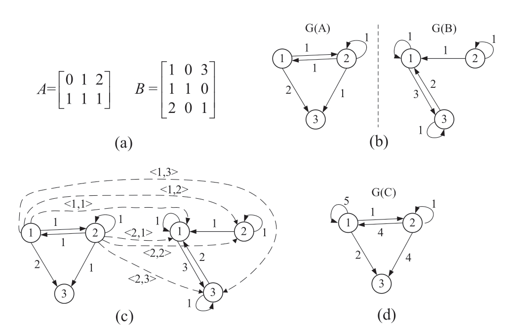
Fig.4 Process of matrix multiplication example

It is clear that the computation for each edge in G(C)is only related to both along with its connected edges in G(A)and along with its connected edges in G(B);however,it is irrelevant to most of the other edges in G(A)andG(B).The topology and edge weights of G(A)and G(B)remain unchanged during the computation,and the newly generated edges are independent of each other.Consequently,the parallel computation can be applied to matrix multiplication.The details are discussed in Section 3.

2.3.2 Graph description of matrix decomposition

When solving a system of equations in the form of Ax=b,matrix decomposition is often used to speed up the solution because of the high time complexity of matrix inversion.Matrix decomposition methods include LU decomposition,Cholesky decomposition,QR decomposition,etc.Generally,existing methods decompose matrix A into the form of the product of two matrices.These methods operate on a single matrix,so the process can be described as a graphG(A).

LU decomposition can decompose a square matrix A into a dot product of a lower triangular matrix L and an upper triangular matrix U,i.e.,A=LU.Since the diagonal elements of matrix L are all zero by default,only one matrix can be used to represent the lower triangle of L(excluding diagonal elements)and the upper triangle of U.From the perspective of graph description,only one corresponding graph is needed to store both the matrix and the resulting values from its subsequent decomposition,where the entire decomposition process can be performed in the graph.The decomposition process primarily amends the value of each vertex in ascending order by vertex index.The amendment has three steps as follows.

Step 1:Amend neighbor-edges.For each vertex p in the graph,we first amend the outgoing neighbor-edges of p.The amendment equation is expressed in(3),which means that the weight of each outgoing neighbor-edge of p is divided by that of self-edge of p.As shown in Fig.5,are examples.

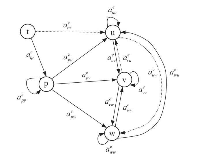
Fig.5 Amendment for vertices

Step 2:Amend self-edges.The self-edge of each neighbor pointed by p is amended as in Fig.5,and the equation is expressed in(4).

Step 3:Amend mutual-edges.For the mutual-edges of p to be amended,such as all edges between the three vertices u,v and win Fig.5.The amendment formula is shown in(5).

Note that for the mutual-edges that do not exist in the original graph(e.g.,the edges of dotted line shown in Fig.5),if the edge weights are not equal to 0 after amendment mutual-edges,it is necessary to add these new mutual-edges to the graph.For those non-diagonal elements in the matrix that are originally 0 and change into non-zero because of matrix decomposition,these elements are defined as injectors in this paper,and the edges corresponding to these injectors are called injected-edges.

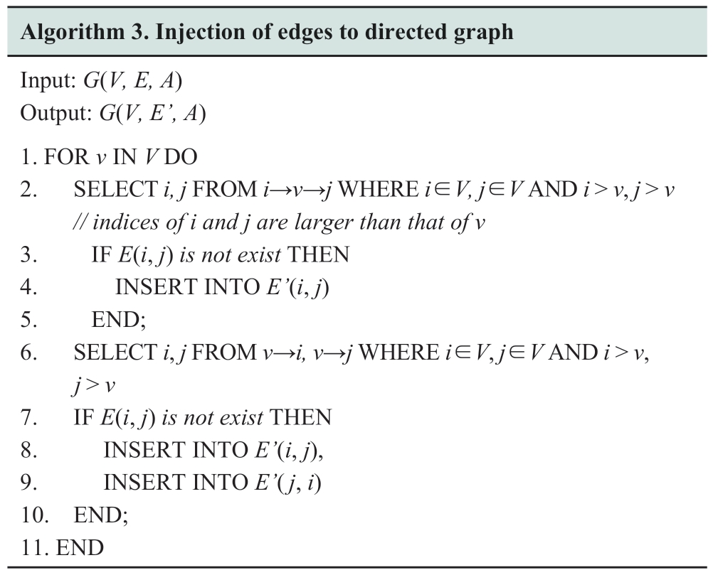
Generally,the number and position of injectors(injectededges)can be determined before matrix decomposition.Subsequently,the operation of insertion of injected-edges is required before decomposing the graph.The insertion process of injected-edges is outlined in Algorithm 3.In line 2,the expression i→v→j is a path in graph G that sources from i to j through the intermediate vertex v.Similarly,the expression v→i and v→j indicate paths pointing from v to i andj,respectively(line 6).Following the edge injection process,the number of vertices and the weights of edges of the graph remain unchanged,whereas the number of edges increases.In other words,the graph G evolves from G(V,E,A)toG(V,E’,A)after the operation.

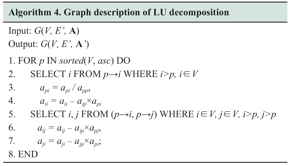
The LU decomposition process is outlined in Algorithm 4,where lines 2 to 4 correspond to the amendment of neighbor-edges and self-edges,and lines 5 to 7 correspond to the process of mutual-edges.In line 1,the functionsorted(V,asc)means that the vertex set V is sorted in ascending order by vertex index,as the vertices in V need to be traversed in order.

Cholesky decomposition decomposes the matrix into the product of upper triangular matrix and lower triangular one.Therefore,the logic of LU decomposition in Algorithm 4 still applies to it except for a few differences in the calculation steps.

Based on this section,matrix multiplication and matrix decomposition operations can be performed by modeling the data into a graph,so that these regular matrix computations can be performed on top of a graph database.In the proceeding section,we will verify the computational performance of the proposed graph description method for matrix operations.

3 Matrix operations on the graph description method

The matrix computation scheme proposed in the above section can be deployed in two approaches.First,by secondary development on open-source graph databases,which modifies the corresponding underlying arithmetic implementation.Second,a computation process is conducted as procedural query steps in any database that supports UDF(user-defined function)or stored procedures.The latter is widely acceptable;however,it is slightly weaker than the former in terms of performance optimization.To verify the effectiveness of the graph description method,we follow the weaker deployment strategy,which is more revealing,and conduct experiments on top of TigerGraph,one of the most versatile graph databases1For other graph databases,the methods designed in this paper can be applied through user-defined functions or stored procedures,as long as they meet the requirements of supporting conventional scientific computation and set structure types,and can store query results in variables that are used for subsequent computations..

TigerGraph is a native graph database with an architecture that supports massively parallel processing.Moreover,the query language of TigerGraph,called GSQL,is a Turing-complete language that enables rich query functions[26].In this section,we implement two common matrix calculations,i.e.,matrix multiplication and LU matrix decomposition,based on the graph description method(referred to as the GD method in the remainder of this paper)on TigerGraph.The effectiveness of the method is verified by comparing with two baselines,i.e.,Python and GSQL implementations,on the time overhead scale.For the Python baseline,all validations were set up without using a third-party library and are implemented natively in the language to facilitate a fair comparison.For GSQL,the computation process is performed entirely in the graph database.The queried data is stored in an internal array and computed using the same algorithm logic as the Python one.

In most practical application scenarios involving matrix computation,such as image processing[27],power grid computation[28],signal processing[29],etc.,the matrices are often extremely sparse,so the experiments covered in this paper are assumed to be sparse matrices.The specific experimental settings are detailed in the following subsections.The same hardware environment is used for all implementations,as listed in Table 2.

Table 1 Parameters of the matrix multiplication example

Table 2 Experimental hardware environment

3.1 Comparison of matrix multiplication

First,we compare the efficiency on the GD method and two counterparts by varying matrix sizes.Two matrices A∈ℝm×n and B∈ℝn×l are randomly generated with different sizes.For a more comprehensive comparison,this experiment is divided into three dimensions.Specifically,two parameters of m,n or l are fixed while the other one is varied to illustrate the influence on different matrix sizes.The sparsity factor α(i.e.,the ratio of the number of nonzero elements in the matrix to the total number of elements)of both matrices A and B is set to α≈0.03.

Figure 6 illustrates the computation time in matrix multiplication of the three methods for different data sizes.In Fig.6(a),we vary m after setting n=800 and l=1200.The result exhibits that the GD method performs the best among the three methods,and its computation time grows more slowly as the data size increases.The execution time of the Python method is significantly longer than those of the other two graph database-based methods.It could be attributed to the underlying computation implementation of the graph database is written in C++ and the query functions are compiled before execution,which enables faster execution compared to the Python interpreted language.

Fig.6 Running time of matrix multiplication

Figure 6(b)exhibits a similar trend as in Fig.6(a),where the value of l increases and m and n remain unchanged at 1,200 and 800,respectively.The GD method shows the best scalability,and the graph database-based methods are still better than the Python method.In Fig.6(c),we vary n and keep both m and l constant at 2,000.Unlike the cases in Fig.6(a)and 6(b),the running time of the Python and GSQL methods gradually grows with the increase of data size.However,the time cost of GD tends to be constant regardless of the value of n.Based on the above results,the GD method is superior to the counterparts in matrix multiplication and has an outstanding computational performance potential for complex calculations,such as matrix dimensionality reduction.

3.2 Comparison of matrix decomposition

The GD method proposed in this paper can implement conventional matrix decomposition algorithms,such as LU decomposition,Cholesky decomposition,etc.In the set of experiments,we consider LU decomposition as an example,where the sizem of a randomly generated matrix A∈ℝm×m is varied to investigate the effect on the efficiency.Similar to the previous experiments,the sparsity factor of A is set to α≈0.03.

Figure 7 illustrates the running time of the three methods in LU decomposition with different matrix sizes and reports that the results are qualitatively similar to Fig.6.As depicted in Fig.7,the GD method outperforms the other two,and the growth rate of its computational cost is relatively flatter as the matrix size grows.Remarkably,the GD method has an obvious advantage in matrix decomposition,particularly for larger graphs.

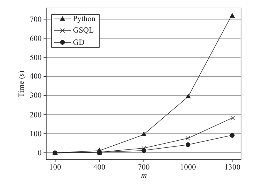
Fig.7 Running time of matrix decomposition

4 Parallel computing based on graph hierarchy

In matrix operations,the required neighbors of each vertex can be quickly queried by the graph structure;thus,it is unaffected by zero elements in the computation.Simultaneously,the reduction of useless loop traversals makes it advantageous in sparse matrix computation scenarios,which is one of the principal reasons why the GD method is significantly better than the other two methods.

Another important reason is benefitting from the parallel nature of the graph database.The GSQL query language of TigerGraph has an integrated parallel indicator called ACCUM.Based on the results of each matched query schema,the indicator can divide the computational tasks to be executed into multiple subtasks and simultaneously execute them using a multi-thread mechanism.For this parallel pattern,there should be no dependency among the computational tasks.Considering matrix multiplication as an example,when each element cij in matrix C is independent of each other,and its calculation involves only the vertices i and j,as well as their respective neighbors,in matrices A and B,the ultimate result is unaffected by the order of calculation.As a result,the computation is highly parallelizable when using the GD method.

In contrast,for matrix decomposition,the computational results of certain vertices affect the subsequent calculation,which makes the progress less parallelizable.A hierarchical parallel computation method based on graph database was proposed in[30],which is based on the elimination tree theory[31].The elimination tree is constructed based on the dependencies between vertices.The vertices at the same layer of the elimination tree are mutually independent,so the calculation can be executed in parallel.The hierarchical strategy can better exploit the parallelism capability of graph databases.Inspired by[17],this study introduces a hierarchical parallel computing method in the matrix decomposition process.Below in Fig.8,we implement the proposed parallel computation based on TigerGraph to verify the efficiency.

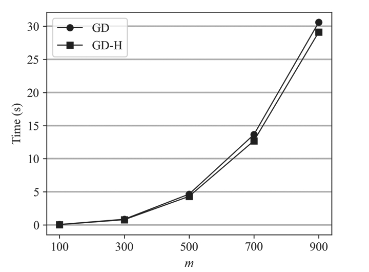
Fig.8 Effect of matrix decomposition with hierarchical parallel

The iteration-based method does not have parallelism;therefore,only the method based on the GD method is retained for this experiment.Figure 7 illustrates the time overhead in matrix decomposition of the GD method following the introduction of hierarchical parallel computing,referred to as the GD-H method,compared with that of the plain GD method.Similar to the above experiments,the data sparsity factor of symmetric matrix A∈ℝm×m is still approximately 0.03.It can be observed that the GD-H method outperforms the plain GD method in terms of time and cost;however,the performance improvement is relatively limited.

To investigate the reasons that influence the efficiency of the hierarchical parallel computation,we explore the effect of different sparsity factors on the number of layers,which is the depth of the elimination tree and directly affects the hierarchical parallelism.We denote the elimination tree generated from the matrix A and the number of layers of the tree as T(A)and TL(A),respectively.We compare TL(A)by varying the matrix sparsity factor α while retaining the data size m of A at 800.

As shown in Fig.9,where Fig.9(b)shows the amplificated image of the curve corresponding to the sparsity factor ranging 0～0.03 in Fig.9(a),it can be inferred from the experimental results that the sparser the matrix,the smaller the depth of the elimination tree,which results in better parallelism.The reason because a smaller TL(A)means that additional vertices can be computed simultaneously within each layer of elimination tree T(A).As shown in Fig.9(a),when the sparsity factor is greater than 0.03,the value of TL(A)tends to coverage to the number of vertices of T(A),i.e.,the elimination tree degenerates from a tree structure to a linear one,which explains why the hierarchical parallelism of GD-H in Fig.8 is not significant for the efficiency improvement.Conversely,when the sparsity factor is less than 0.015,as shown in Fig.9(b),the elimination tree can obtain a smaller depth with a superior hierarchical parallel effect.

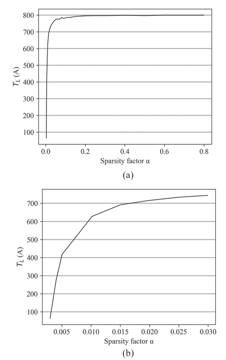
Fig.9 Effect of the sparsity factor on TL(A)

5 Power flow based on the graph description method

Power flow computation is one of the most fundamental and important calculations in power system analysis.The task of power flow is to determine the power distribution and power losses in the grid,as well as the voltage at each bus,according to the given operating conditions.The core of power flow computation primarily includes the following three steps:1)generation of the nodal admittance matrix and Jacobi matrix;2)calculation of the active and reactive power variations from the nodal power equation;3)and the iterative solution of the voltage phase and amplitude corrections from the Jacobi matrix.The evaluations of the admittance matrix and the Jacobi matrix are only related to the corresponding bus nodes and neighbor nodes,and the value of each node does not change during the calculation.Hence,the values in the two matrices can be calculated simultaneously.The same applies to the calculation of active and reactive power variations.In other words,the above calculations fully exploit the parallel mechanism of the graph database.The iterative process of Jacobi in the power flow computation is primarily the matrix operation,as shown in(6)(the notations in the equation can be referred from[32]).

Based on the graph description method proposed in this study,the above steps of power flow computation can be performed in the graph database.Accordingly,we implement the power flow computation based on the graph description method on top of graph database,which verifies the practicality of the proposed GD method.The experiments use two datasets of power data,i.e.,IEEE 118-node test case and Central Europe 1354-node power system[33],both of which are from the MATPOWER test cases and in the same data form.The former case contains 54 generators and 186 branch lines,and the later contains 260 generators and 1991 branch lines,with a rated capacity of 100 MVA for both cases.

When constructing the heterogeneous graph of power grid,buses and generators are abstracted as vertices in the graph model.Parameters such as power,voltage,and load are considered as attributes stored in the vertices.The grid lines and transformers are simplified as edges of the graph,and the attached parameters,such as resistance,reactance,and admittance are modeled as attributes of the edges in the graph.Thus,the concrete power grid can be transformed into a topology graph.

Given that the Jacobi matrix in the PQ decomposition method remains unchanged during the calculation and only one matrix decomposition is required,the PQ method is a faster solution.Therefore,the PQ decomposition method is more desirable in this experiment,and we selected it for the power flow computation.Concerning matrix solving,although there are multiple matrix decomposition methods,LU decomposition is chosen owing to its looser usage restrictions as the matrix decomposition implementation component.To optimize the solution efficiency,this application combines the GD method and GSQL language to solve the system of equations.The power flow calculation follows the process described in[32],whose steps conducted using graph description-based query and computing are as follows:1)Reorder the index numbers of PQ and PV nodes after dividing by the node type;2)Query each edge to perform the admittance calculation and accumulate the result to the target node element in the admittance matrix pointed by the source node;3)Query the power and load of each generator,and then calculate the initial injected power of each node;4)Query each edge to determine the node type(PQ or PV)at its two ends,and then calculate the values of the H and L matrices of the Jacobi matrix;5)Perform the decomposition of H and L matrices separately using the method described in Section 2.3.2;6)Query the voltages and phase angles at the two ends of each node,and then update its power with the admittance matrix;7)Query the injected power of each node to obtain the amount of power imbalance,and then retrieve the maximum imbalance;8)Based on the decomposition matrices of H and L,calculate the corrections of the voltage and phase angle using the forward and backward substitution method,and then query and update each node;9)Repeat steps 6-8 until convergence.

As a control group,two calculation tools,i.e.,MATLAB and Python,which are conventional for power grid computation,were used to implement the same arithmetic logic as the graph description method to demonstrate the efficiency comparison.Meanwhile,for comparison with relational databases,we constructed the power grid schema based on MySQL.To ensure fairness,it used the same PQ decomposition method as the GD one.Table 3 lists the flow calculation results of voltage magnitude and phase angle of six arbitrarily selected nodes for the 118-node case as samples based on our proposed method.The three experimental comparison methods show the same results because they use the same algorithm logic.Moreover,the results are basically the same as those of Pypower,a thirdparty library for power grid computation in Python.

Table 3 Voltage and phase angle results for some nodes in flow computation

Figure 10 illustrates the time cost of different computation methods after the same number of iterations.To better examine the scalability for different grid topologies,we supplement the 2383-node dataset,which comes with the MATPOWER software.The results reveal that when the graph dataset size is small,all three methods can complete the computation in a relatively short time.In contrast,as the data volume increases,the proposed graph description method can obtain a significant performance advantage compared to the other three counterparts.The result shows that the proposed method is completely valuable for practical application.Notably,when the number of nodes increases,the performance of MATLAB by virtue of the underlying computation optimization improves.For relational MySQL,iterative queries in the PQ method result in a significant degradation,which conforms with the results in[20].

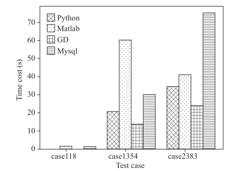
Fig.10 Comparison of power flow computation

Furthermore,we performed N-1 contingency analysis based on the graph description in the following three steps:1)Randomly select a single branch or generator to drop from the grid,namely set the “working” attribute of the corresponding edge or node from 1 to 0;2)Recalculate the flow using the graph description method;3)Determine whether the flow results are stable or exceed the rated values according to the rated capacity of each line and the rated voltage/power of each device.The experiment results of N-1 contingency computation are qualitatively similar to those of the comparison experiment on the flow calculation,due to space constraint,we do not report them in detail.

Based on the proposed graph description method,power analysis tasks,such as power loss and voltage crossing detection,can also be implemented.However,applying graph databases to actual power systems still faces limitations.For instance,the data of EMS and other power systems are basically stored in the relational model,and are an important asset in power systems.In addition to being costly,data migration and data structure changes could also result in uncertain risks.On the contrary,for new power subsystems,such as new distribution grids,power market systems,and systems with more nodes or dynamics,they may be more appropriate to use graph databases in the future to bring the advantages of graph computing into play owing to relatively less data accumulation.

6 Conclusion

Graph structures are well suited for expressing interentity association relationships and handling multi-source heterogeneous data.Combined with the advantages of graph databases in data management,modeling,and parallel computation,they can be used in power systems.Existing researches on power grid computation primarily utilize hardware platforms to enhance computational efficiency.Nevertheless,they typically only make use of the graph database features of modeling heterogeneous data and efficient data retrieval,whereas the computation process still needs to be migrated outside the database and thus cannot avoid expensive I/O overhead.Based on the correlation between a graph and matrix,this study proposes a method based on graph description to complete matrix operations and parallel computing.The proposed method fills the gap of existing graph databases that lack the native interface or internal support of matrix operation,enabling many computation tasks to be placed inside the graph database,extending the scope of application.In the experiments,the graph description method exhibits obvious advantages over the baselines in typical power system scenario,i.e.,power flow calculation and N-1 contingency computation tasks.The experimental results demonstrate the effectiveness of our proposed method.In future research,we will continue to explore more feasible scenarios in the field of power systems.

Acknowledgements

This work was supported by the National Key R&D Program of China(2020YFB0905900).

Declaration of Competing Interest

We declare that we have no conflict of interest.

References

[1]Bhattarai B P,Paudyal S,Luo Y,et al.(2019)Big data analytics in smart grids:state-of-the-art,challenges,opportunities,and future directions.IET Smart Grid,2(2):141-154

[2]Wang L,Shang L,Ma M,et al.(2018)Fault diagnosis and trace method of power system based on big data platform.IOP Conference Series:Materials Science and Engineering,394(4):042116

[3]Wang F,Shi J,Ju X,et al.(2018)An efficient graph data processing framework for power grid systems.Proceedings of 2018 IEEE SmartWorld,Ubiquitous Intelligence &Computing,Advanced &Trusted Computing,Scalable Computing &Communications,Cloud &Big Data Computing,Internet of People and Smart City Innovation,Guangzhou,China,Oct 2018

[4]Percuku A,Minkovska D,Stoyanova L(2017)Modeling and processing big data of power transmission grid substation using Neo4j.Procedia Computer Science,113:9-16

[5]Kan B,Zhu W,Liu G,et al.(2017)Topology modeling and analysis of a power grid network using a graph database.International Journal of Computational Intelligence Systems,10(1):1355-1363

[6]Cheng Z,Zhong T,Zhang S,et al.(2022)Survey of recommender systems based on graph learning.Computer Science,49(9):1-13

[7]Rashmi R,Champawat S,Varun Teja G,et al.(2020)Analysis of road networks using the Louvian community detection algorithm.In:Das K,Bansal J,Deep K,et al.(eds)Soft computing for problem solving.Advances in Intelligent Systems and Computing,1057,Springer,Singapore,749-757

[8]Lysenko A,Roznovat I A,Saqi M,et al.(2016)Representing and querying disease networks using graph databases.BioData Mining,9:23

[9]Xie K,Zhang H,Hu B,et al.(2010)Distributed algorithm for power flow of large-scale power systems using the GESP Technique.Transactions of China Electrotechnical Society,25(6):89-95

[10]Wei G(2022)Research on parallel power flow computing in power grids based on GPU.Dissertation,Northeast Electric Power University

[11]Yang G,Yu L,Liu M(2013)A method for accelerating power flow calculation based on multiple light threads.Power System Technology,37(6):1666-1671

[12]Zhang D,Yan Z,Xu X,et al.(2016)Large-scale Ill-conditioned power flow calculation using implicit Cholesky factorization method.Power System Technology,40(4):1197-1203

[13]Liu Z,Chen Y,Song Y,et al.(2020)Batched computation of continuation power flow for large scale grids based on GPU parallel processing.Power System Technology,44(3):1041-1046

[14]Blalock D,Guttag J(2021)Multiplying matrices without multiplying.doi:10.48550/arXiv.2106.10860

[15]Fawzi A,Balog M,Huang A,et al.(2022)Discovering faster matrix multiplication algorithms with reinforcement learning.Nature,610:47-53

[16]Zhou S,Kannan R,Prasanna V K(2020)Accelerating stochastic gradient descent based matrix factorization on FPGA.IEEE Transactions on Parallel and Distributed Systems,31(8):1897-1911

[17]Dai J,Chai B,Qiu H,et al.(2016)Analysis of distribution network outrage region based on graph database.Proceedings of China International Conference on Electricity Distribution,Xi'an,China,2016

[18]Jiang W,Wang M,Chen J,et al.(2022)Calculation of power supply reliability for distribution network based on Neo4j graph database.Automation of Electric Power Systems,46(15):104-111

[19]Zhao Y,Yuan C,Liu G,et al.(2018)Graph-based preconditioning conjugate gradient algorithm for “N-1”contingency analysis.Proceedings of 2018 IEEE Power &Energy Society General Meeting,Portland,OR,USA,2018

[20]Liu G,Dai R,Lu Y,et al.(2020)Graph computing based power network analysis applications.Transactions of China Electrotechnical Society,35(11):2339-2348

[21]Cheng Y,Ding P,Wang T,et al.(2019)Which category is better:benchmarking relational and graph database management systems.Data Science and Engineering,4(4):309-322

[22]Fang X,Huang J,Wang F,et al.(2020)ConSTGAT:contextual spatial-temporal graph attention network for travel time estimation at Baidu Maps.Proceedings of the 26th ACM SIGKDD International Conference on Knowledge Discovery &Data Mining,New York,NY,USA,Aug 2020

[23]Yin X,Wu G,Wei J,et al.(2021)Multi-stage attention spatialtemporal graph networks for traffic prediction.Neurocomputing,428:42-53

[24]Wang H,Kong H,Li X(2021)User’s home location prediction based on filtered text and social networks.Journal of Geo-Information Science,23(10):1778-1786

[25]Jiang W,Wang M,Chen J,et al.(2022)Calculation of power supply reliability for distribution network based on Neo4j graph database.Automation of Electric Power Systems,46(15):104-111

[26]Deutsch A,Yu X,Wu M,et al.(2019)TigerGraph:a native MPP graph database.doi:10.48550/arXiv.1901.08248

[27]Elad M,Figueiredo M A T,Ma Y(2010)On the role of sparse and redundant representations in image.Proceedings of the IEEE,98(6):972-982

[28]Karimipour H,Dinavahi V(2015)Extended Kalman Filter-based parallel dynamic state estimation.IEEE Transactions on Smart Grid,6(3):1539-1549

[29]Brown I J(2009)A wavelet tour of signal processing:the sparse way(3rd Edition),Academic Press,FL,United States

[30]Dai R,Liu G,Wang Z,et al.(2020)A novel graph-based Energy management system.IEEE Transactions on Smart Grid,11(3):1845-1853

[31]Liu J W H(1990)The role of elimination trees in sparse factorization.SIAM Journal on Matrix Analysis and Applications,11(1):134-172

[32]Meng X,Gao Y(2010)Power system analysis(2nd Edition).Higher Education Press,Beijing

[33]Josz C,Fliscounakis S,Maeght J,et al.(2016)AC power flow data in MATPOWER and QCQP format:iTesla,RTE Snapshots,and PEGASE.J,doi:10.48550/arXiv.1603.01533

Received:9 October 2022/Accepted:27 December 2022/Published:25 Feburary 2023

Daoxing Li

lidaoxing@epri.sgcc.com.cn

Kai Xiao

xiaokai1@epri.sgcc.com.cn

Xiaohui Wang

wangxiaohui@epri.sgcc.com.cn

Pengtian Guo

guopengtian@epri.sgcc.com.cn

Yong Chen

ychen@epri.sgcc.com.cn

2096-5117/© 2023 Global Energy Interconnection Development and Cooperation Organization.Production and hosting by Elsevier B.V.on behalf of KeAi Communications Co.,Ltd.This is an open access article under the CC BY-NC-ND license(http://creativecommons.org/licenses/by-nc-nd/4.0/).

Biographies

Daoxing Li received his master’s degree at North China Electric Power University,Beijing,in 2021.He is working in China Electric Power Research Institute Co.,Ltd.His research interests include artificial intelligence and graph computing.

Kai Xiao received his master’s degree at North China Electric Power University,Baoding,in 2013.He is working in China Electric Power Research Institute Co.,Ltd.His research interests include power big data technology,graph computing and marketing business.

Xiaohui Wang received the Doctor’s degree from North China Electric Power University,Beijing,2012.He is currently working at the China Electric Power Research Institute Co.,Ltd.Beijing.His research interests include power big data technology,artificial intelligence,active distributed network,energy internet.

Pengtian Guo received his master’s degree at North China Electric Power University,Beijing,in 2020.He is working in China Electric Power Research Institute Co.,Ltd.His research interests include power Internet of things and artificial intelligence.

Yong Chen received the Doctor’s degree from Huazhong University of Science and Technology,Wuhan.He is working in China Electric Power Research Institute Co.,Ltd.His research interests include high performance computing,artificial intelligence.

(Editor Yajun Zou)