0 Introduction

The accurate determination of the causes of transmission line faults is extremely important.It supports grid operation and maintenance personnel in formulating targeted maintenance strategies to prevent the further deterioration of line conditions [1].Hence,it aids in preventing grid collapse and large-scale power outages [2-3].Furthermore,accurately identifying the causes of transmission line faults is relevant in the development of late line defense plans and incident drills.In view of the goal of achieving “carbon peak and carbon neutrality”,new methods for energy generation have rapidly developed,and the proportion of wind power and photovoltaic access has increased.However,the increase in the uncertainty of system states,incorporation of more fragile components,and high complexity in fault modes and characteristics require improvements in identifying transmission line faults.

Traditional fault identification methods mainly rely on fault detection elements and identification criteria.In these methods,reasonable identification criteria are set based on the comprehensive analyses of fault mechanism and waveform characteristics [4-5].In reference [6],different waveform characteristic parameters from the frequency,temporal,and arc domains were proposed.Furthermore,identification criteria were established via the multiparameter fusion method to identify the various causes of line faults.In reference [7],the line waveforms of non-fault lightning strikes,fault lightning strikes,and ordinary shortcircuit faults were investigated; the identification criteria for the three transient processes were proposed.In reference [8],statistics on line wildfire tripping and fault characteristics were combined to identify wildfire tripping accidents based on pre-discharge current and traveling wave fault characteristics before tripping.Furthermore,in reference[9],short-circuit faults due to external factors,such as birds and animals,tree branches,lightning strikes,and cables,were examined.In the study,voltage and current waveform characteristics were assessed with respect to various fault types.Moreover,the correlation between waveform characteristics and fault causes were evaluated.The criteria for classifying and identifying different fault causes were also developed.In reference [10],transient symmetrical components were used to characterize the transmission line fault waveforms.The waveform and external environment features were identified based on the fault waveform database and formulated identification criteria,respectively.

Traditional fault identification methods are easily affected by the system run mode,fault positioning,transition resistance,new energy access ratio,and other factors; consequently,they lose their effectiveness.Furthermore,subjective factors that influence identification outcomes exist.Given that new energy-consuming equipment is widely connected and the proportion of new energy sources continues to increase,the corresponding relationship between the power system and fault waveform characteristics can potentially change to a certain extent.In turn,this can influence the effectiveness of traditional identification methods.In recent years,intelligent algorithms have been rapidly developed and gradually applied to transmission line fault identification.Furthermore,certain research results have been obtained [11-17].The use of intelligent algorithms can effectively overcome the excessive dependence on prior knowledge.Furthermore,these algorithms are less affected by parameters,system run mode,fault positioning,and new energy access ratio.

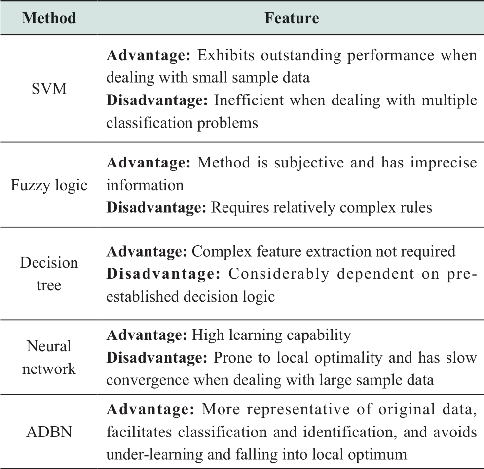
However,the intelligent classification and identification algorithms based on existing fault identification methods have certain limitations.Specifically,the fuzzy logic method requires relatively complex rules with high robustness[18].The decision tree method considerably relies on preestablished decision logic [19-20].The neural network method is prone to local optimality and slow convergence when dealing with large sample data [21].The support vector machine(SVM)method is relatively inefficient when dealing with multiple classification problems[22].Additionally,the current fault identification models based on intelligent algorithms are mainly classified from the perspective of fault routing according to waveform features.However,the intrinsic correlation between waveform features and fault causes has not been explored in depth.

With the persistently increasing proportion of gridconnected new energy sources,the waveform characteristics of power system faults are becoming more complicated.Hence,the correlation between the causes of faults and waveform characteristics is difficult to characterize.Moreover,the existing identification algorithms lack applicability.A deep learning structure can more representatively characterize the knowledge conveyed by massive data than the traditional intelligent algorithm.However,when the number of data samples is insufficient,obtaining optimal results using a deep learning structure via training may be difficult.The deep belief network(DBN)model emerged in 2006 [23-24].Previous studies have shown that this model is considerably capable of extracting sample features and has fault-tolerance characteristics.The model can be used to effectively solve classification and identification problems involving samples via layer-by-layer training.

In the context of “carbon peak and carbon neutrality”,the uncertainty of the power system increases,and the relationship between the electrical characteristics of faults and their causes becomes more complex.In Western China,the construction of large-scale wind and solar bases has accelerated,and in Eastern China,the development of distributed new energy and offshore wind power has continued.In view of the high proportion of new energy access to the grid,the assessment of power system faults is confronted with certain challenges.The output of new energy units has fluctuation characteristics,and the power generated by new energy units in different regions has certain temporal and spatial correlations.

A regional power grid connected to new energy units on a large scale has a certain impact on key electrical quantities in the power system.This results in increasingly complex fault characteristics that create confusion in the corresponding relationship between fault causes and electrical quantities.Because of the foregoing reasons,the traditional fault identification methods may be unsuitable for scenarios where the proportion of new energy connected to the grid is high.

In this study,a transmission line fault identification method applicable to a high percentage of new energy access scenarios is investigated.For this purpose,the temporal–frequency features of fault waveforms,new energy-related parameters,and deep learning models are used.The information on important features related to new energy access to the grid is summarized.The method fully considers the impact of new energy on the electrical quantity for fault identification.The DBN model is upgraded to an adaptive deep belief network(ADBN)model.This increases the speed of model convergence by automatically adjusting the learning step.By combining different fault mechanisms,10 parameters,which are related to the causes of line faults,are selected to generate feature parameters and formulate an ADBN-based model for fault recognition.The validity of the fault recognition model is assessed by utilizing actual data in the model.Furthermore,the fault recognition accuracy is analyzed under varying model/feature parameters,sample set sizes,and proportions of new energy sources.The application results indicate that the proposed model can effectively identify various fault causes,such as tree branches,wildfires,birds and animals,lightning,wind deflection,icing,and external force damage.The model is applicable to scenarios with different proportions of new energy access to the grid.

The rest of this paper is organized as follows.The analysis of the ADBN model is summarized in Section 1.In Section 2,fault diagnosis based on the ADBN model is proposed.The case studies and analysis method are presented in Section 3.Finally,concluding remarks are summarized in Section 4.

1 ADBN model

Similar to the classical DBN architecture,the ADBN model comprises a sequence of restricted Boltzmann machined(RBMs).The DBN framework architecture is described in Fig.1.The RBM is composed of visible(input)and hidden(output)layers that are fully connected bidirectionally.Furthermore,no linkage exists between the two layers.Suppose that vectors v and h denote the states of the explicit element of the visible layer and implicit element of the hidden layer,respectively.Moreover,vi and hj represent the states of the ith explicit element and jth implicit element,respectively.Accordingly,the energy function for a designated set,(v,h),can be formulated as follows [25-27]:

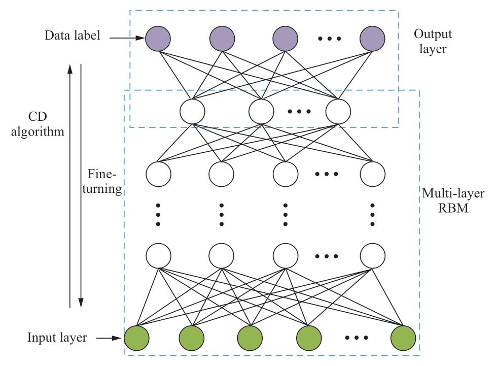
Fig.1 Structure of ADBN model

where θ∈{Wij,ai,bj} denotes the RBM model parameter[29]; a∈Rm and b∈Rn represent the biases of explicit and implicit elements,respectively; and W∈Rn×m refers to the matrix of the connection weight between the explicit and implicit elements [25-27].

The joint distribution of probabilities for every state(v,h)of the visible and hidden layers is formulated as

where Z is the partition function; it can be considered as the aggregation of energy functions under all visible and hidden layer states.Function Z is formulated as

The marginal distribution for the joint distribution of probability P(v,h/θ)is

Because the visible layer has a state,v,the probability of actuation of the hidden layer’s jth element,hj,can be formulated as

Because the hidden layer has a state,h,the probability of actuation of the visible layer’s ith element,vi,can be formulated as

In Equations(5)and(6),σ()represents the activation function,which is typically formulated as

The formulation of criteria for activation and startup is required through threshold settings.These settings are formulated as follows:

where ξ refers to the threshold of probability to distinguish between the on and off neuron states of the hidden layer with the value range 0.5–1 [29].The process given by Equations(5)–(8)is a course of Gibbs sampling.

Following the CD-k criterion [27-28],updating the parameter set,θ∈{Wij,ai,bj},is formulated as

where η denotes the rate of learning.Extensive research has demonstrated that the distribution of visible and hidden layers can be smoothed by setting k=1.

With the CD-k algorithm,multiple iterations are necessary for every RBM,and parameter updating in the identical direction after every iteration is not mandatory[30].Accordingly,if the learning rate is constant,the algorithm is seemingly “premature” or can barely converge.In designing the ADBN algorithm in this study,the learning rate is modified from constant to adaptive.To establish the adaptive learning rate,the similarities and discrepancies in parameter-updating directions between two successive iterations of RBM-based training are exploited.The adaptive learning rate is updated via the following mechanism:

where Δ=(<vihj>0-<vihj>k)×(<vihj>’0-<vihj>’k); α and β denote the increase and reduction coefficients for the learning rate,respectively; and Δ represents the product of parametric fluctuations during two consecutive RBM iterations.In the case of parametric updating in contrary directions following two consecutive iterations,the learning rate declines.Moreover,in the case of parametric updating in identical directions following two iterations,the learning rate increases.The initial state of the input layer is represented by; its reconstruction state following k iterations is represented by.The states of the hidden layer obtained using the initial stateand after kiterations are denoted by,respectively.

In every sampling process,the weight update is proportional to the value of state sampling.During each Gibbs sampling,the weight is updated once.In an interim state,binary sampling is performed twice.Accordingly,the associations ofξ with α and β are α ≈ 2ξ and β ≈ ξ,respectively.Ranges [1,2] and [0,1] are assigned for α and β,respectively.With the use of Equation(12)to achieve adaptive variation in the learning rate,an adaptive alteration in the error correction signal occurs during supervised learning.The foregoing occurs according to the similarities and discrepancies between the directions of two consecutive updates.This accelerates convergence and enhances the accuracy of the CD algorithm.

A comparison of various methods is summarized in Table 1.

Table 1 Comparison of different methods

2 Fault diagnosis based on ADBN model

2.1 Data Sources

Regarding the primary sources of fault data herein,the(1)online monitoring data,(2)tripping reports,(3)and traveling wave fault data of overhead transmission lines(OTLs)where the line voltage level is 110–750 kV are obtained from the State Grid Corporation of China.To determine the traveling wave fault,the distributed system arranged along transmission lines and substations is used.In the tripping report,the faults between 2010–2020 are included.

Based on the foregoing data,a sample set of transmission line faults containing a total of 3121 typical faults is generated.With new energy sources introduced at a high proportion to the grid,significant differences in primary energy characteristics,number of components,component types,and time scales are found in the system.Hence,the causes of faults become more complex,and the existing standards for establishing the correlation between the fault causes and quantitative characteristics of electrical faults are difficult to implement.To identify different types of line faults to the maximum extent possible when the proportion of new energy access scenarios is high,the fault causes are classified into nine categories.The failure area covers different provinces in China and corresponds to different new energy access scales.The distribution of data samples is summarized in Table 2; training data include 80% of the overall samples.Typical waveforms corresponding to different types of faults are shown in Fig.2.The sampling rate of the fault current detection device is 1 MHz.

Table 2 Fault samples used in experiments

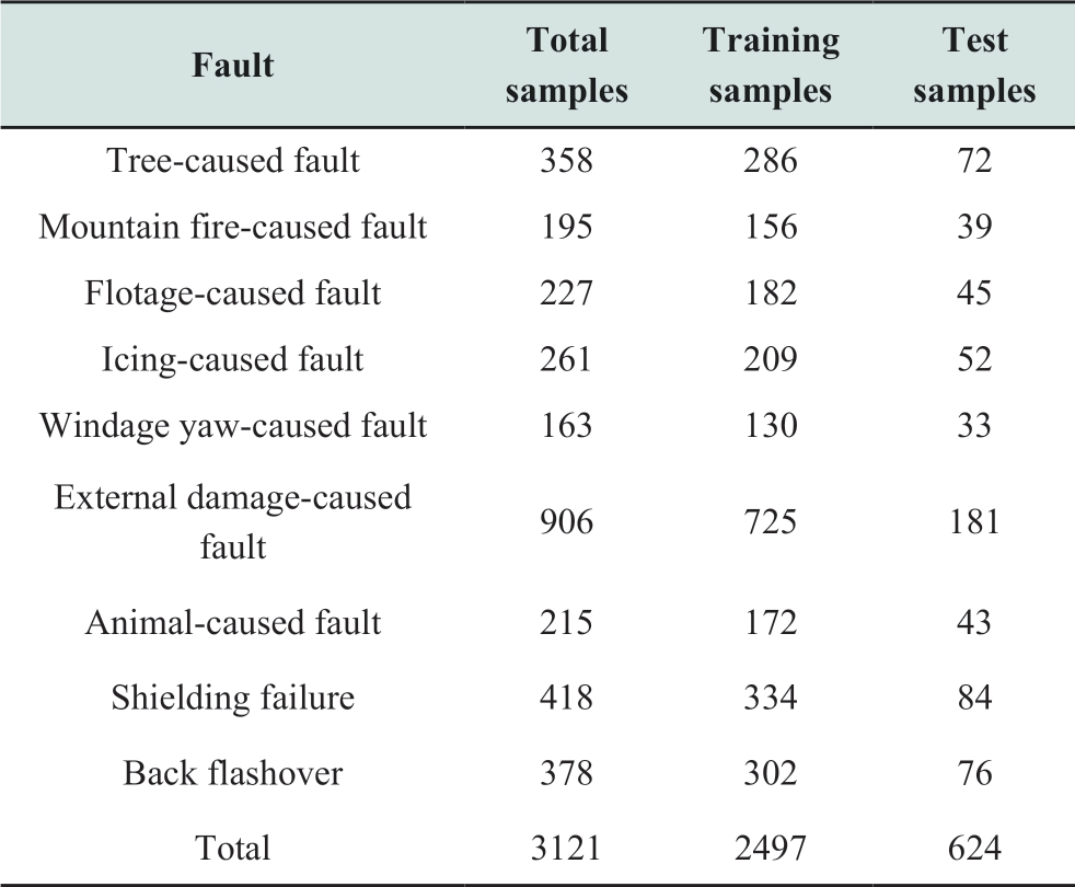
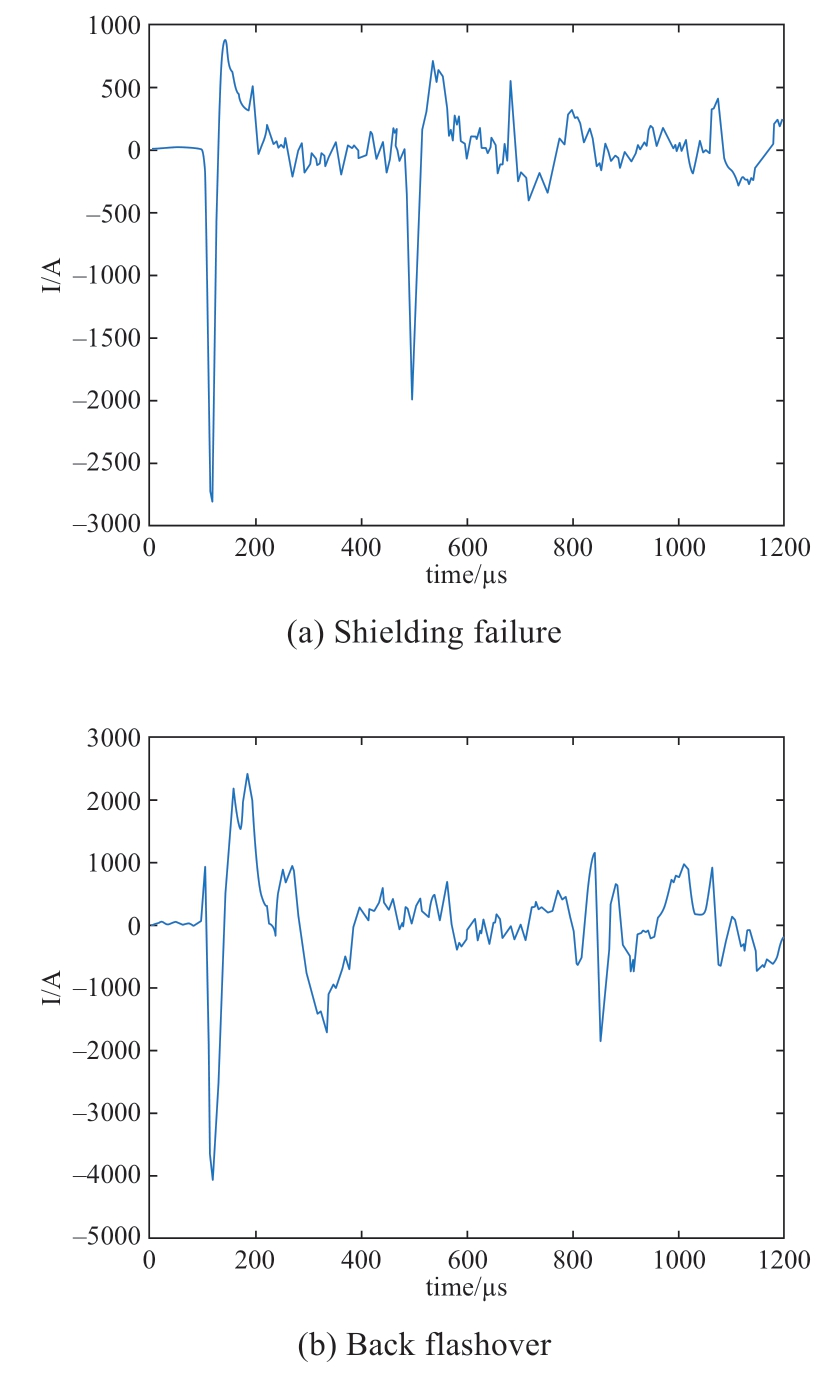
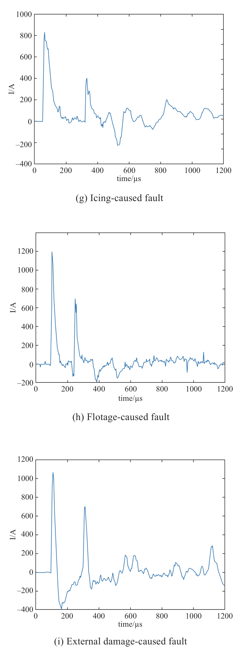
Fig.2 Typical waveforms for different fault types

2.2 Feature parameter selection

Numerous fault-related parameters,such as polarity,amplitude,fault duration,fault position,and transition resistance,are involved in transient traveling waves.Such information offers an important basis for diagnosing faults in OTLs.The temporal frequency features of traveling waves slightly vary according to the type of faults.Based on the time–frequency characteristics of fault waveforms and new energy-related parameters,the study selects suitable temporal frequency feature parameters as the model input for ADBN.

Two types of faults due to lightning strikes may affect OTLs:shielding failure(SF)and back flashover(BF).For these fault types,the wave tail durations of currents are short.In the case of BF,overvoltage has a steep wave head and large amplitude; further,the three-phase voltage varies considerably.After a lightning strike,voltage rapidly increases in the fault phase,leading to insulator flashover.Given the interphase coupling and corona effects,a highfrequency oscillation of the non-fault phase voltage occurs in response to the fault phase voltage.After the fluctuation terminates,the voltage resumes to normal.Because the lightning current in the SF is lower than that in the BF,the SF has a smaller overvoltage amplitude than the BF.Moreover,prior to the insulator flashover,the flow of lightning currents in the SF and BF faults varies in direction.In the SF,the lightning current is injected into the strike point.Following the breakdown of insulation,the lightning current is mostly released to the tower in addition to its partial flow along the conductor.In the BF,the lightning current is released into two parts:tower top-to-corner discharge and line release due to insulation breakdown.Additionally,the flow of lightning current via the arrester occurs prior to insulation breakdown.The induction of a reversed polarity pulse on the faulty line also occurs.The foregoing analysis shows that the traveling wave fault between the BF and SF slightly differs.

The traveling wave current of non-lightning strike fault compared with that of lightning strike fault is smaller in amplitude and has a longer wave tail duration.Thus,the latter can be differentiated from the former based on the half wavelength and amplitude of the traveling wave.The causes of non-lightning faults can also be identified by exploring the transient traveling wave features [31].After analyzing the actual field data and fault mechanism,the following are concluded.

(1)The tree-caused fault(TF)is attributed to the contact between wires and tree branches or inadequate branch–wire distance.Compared with other grounding faults at high impedances,the wave head has a steep rising edge and gentle falling edge.Prior to the primary discharge peak,intermittent flashover occurs.The initial traveling wave has a small amplitude whose minimum value is at the ampere level.

(2)The mountain fire-caused fault(MFF)is mainly attributed to air thermoionization.The wave head’s rising edge and the wave tail’s falling edge are both slow.The initial traveling wave is small in amplitude and has a distinct pre-discharge feature.

(3)The flotage-caused fault(FF)results from the suspension of the floater on the ground wire,conductor,or tower that leads to a lower wire–ground potential than the safe value.The traveling wave has a steep rising edge and large amplitude(up to a few kiloamperes).Bifurcation is typically present in the waveform.

(4)The icing-caused fault(IF)occurs when the insulator surface is covered with ice,compromising the insulation behavior.Prior to the occurrence of IF,the harmonic contents of the waveform are low.The initial traveling wave has a steep rising edge and large amplitude; however,it may be smaller compared with that of other metallic shorted faults.

(5)The windage yaw-caused fault(WYF)occurs due to powerful winds,causing the distance of the wire from the tower/arrester to be shorter than the safety threshold.The waveforms,which have a distinct reflected wave,are extremely similar.The initial traveling wave has a large amplitude.

(6)The external damage-caused fault(EDF)results from the close distance between a crane and conductor.The fault exhibits a metallic short-circuit feature.The rising edge of the wave head is steep.The falling edge of the wave tail refers to the steepest edge in non-lightning faults.The amplitude of the initial traveling wave can be as high as some kiloamperes.

(7)The animal-caused fault(AF)generally occurs when the distance between two conductors is short and the amplitude of the waveform is small.This fault is larger than other high-impedance grounding faults.Moreover,the waveform includes high-frequency harmonic components before and after the flashover.

The foregoing analysis indicates that the waveforms of different fault types exhibit specific differences in amplitude,half wavelength,steepness,energy in diverse periods,and energy in different frequency bands.

When the proportion of new energy access to the grid is high,the physical form and operational features of the power system can evidently be altered.Furthermore,the increase in system complexity,nonlinearity,and uncertainty leads to a certain impact on fault waveform characteristics.Therefore,the correlations among parameters,such as that between new energy access ratio,new energy output rate,new energy penetration rate,and fault waveform characteristics,must be fully considered.In addition to the foregoing,a specific association between fault occurrence time and cause exists.For instance,(1)AF usually occurs during daytime in spring or summer;(2)SF and BF frequently occur during summer nights;(3)TF is regularly observed in autumn;and(4)IF is frequently recorded in winter.Therefore,in addition to waveform features,the model input feature information must be generated.This can be accomplished by combining parameters,such as fault occurrence time,new energy access ratio,new energy output rate,and new energy penetration rate.Note that the wavelet transform has time–frequency window adaptivity and can completely exhibit the feature information of a signal at different scales.Accordingly,cubic B-spline wavelets [32] are used in this study to decompose and reconstruct the traveling waveform signal.The characteristic parameters are chosen as follows:

where T refers to the characteristic vector; f(t)represents the traveling wave signal obtained in the fault phase; and T0 denotes a three-digit binary number indicating the fault occurrence time(the first two digits indicate the season(00-spring,01-summer,10-autumn,and 11-winter),and the last digit represents day or night(0-day and 1-night)).The start and end times of the selected waveform are represented by t0 and ttotal,respectively.The start and end times of the initial traveling wave are denoted by ts and tw,respectively.Half of the total sampling time is denoted by tmid,and tk represents the characteristic moment and indicates a self-defined value ranging between tmid and ttotal(this time is mostly adopted for comparing the time–frequency characteristics before and after the initial wave head).Im refers to the peak value of the initial wave head;tm indicates the time consistent with the peak value; and th is the time consistent with the half-peak value(th > tm).The wavelet decomposition level is indicated by n; Ei represents the energy in the ith frequency band after wavelet transform,and its time range is [ts,tw]; ej represents the energy in the jth frequency band after wavelet transform,and its time range is [t0,tk]; and U0 is the line voltage.The ratio of the maximum steepness of the wave head to the line voltage is denoted as Ms; T8 and T9 are composed of several parameters in which µ0 is used to describe the functional location of the area where the fault occurs(the value is either 1 or 0:1-sending end,0-receiving end).The proportion of new energy generation in the area where the fault occurs in the total power generation is denoted as ω0;ω1 indicates the utilization rate of new energy in the area where the fault occurs; ωmax denotes the maximum ratio of new energy power fluctuations to the load in the area where the fault occurs; λ1denotes the ratio of the installed capacity of the internal use new energy to the internal load power in the area where the fault occurs; and λ2 denotes the ratio of the installed capacity of the outgoing new energy to the outgoing channel power in the area where the fault occurs.

In Equation(14),parameters T1,T2,and T7 denote the time domain energy characteristics of different intervals of the waveform; parameters T3 and T4 denote the amplitude and steepness characteristics of the different intervals of the waveform,respectively; parameters T5 and T6 denote the frequency domains of different intervals of the waveform;and parameters T8 and T9 denote the characteristics related to new energy access to the grid.A softmax classifier is adopted for the output of ADBN.In terms of n independent classifications,the consistent labels for output are set to 1,2,...,n.Each label is consistent with one category.The maximum value of n outputs(normalized between 0 and 1)can be set to 1,and the rest of the output values can be set to 0.With the output value being 1,the consistent label represents an ideal category.In this study,the labels corresponding to the fault causes are set as 1-TF,2-MFF,3-FF,4-IF,5-WYF,6-EDF,7-AF,8-SF,and 9-BF.

The training process of the proposed diagnosis model and the overall framework of the proposed method are presented in Figs.3 and 4,respectively.

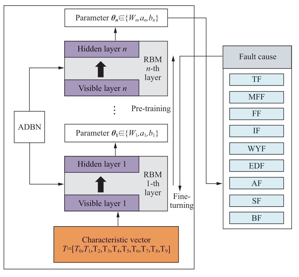
Fig.3 Training process of fault identification model

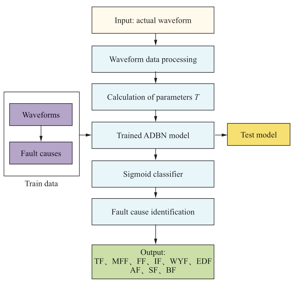
Fig.4 Overall framework of proposed method

The fault identification steps are as follows.

(1)Extract the fault waveform data corresponding to the different fault causes.

(2)Calculate the time–frequency characteristic information,T,of the fault waveform,and use T as the input characteristic parameter of the ADBN model.

(3)Train the ADBN model layer by layer.In the training process,the algorithm can adjust the learning rate according to the similarities and differences in iteration directions of model parameters.After the initial training of the parameters,the backpropagation algorithm fine-tunes the network parameters.

(4)Test the data based on the trained model.

(5)Input new waveform data and output fault cause.

3 Case studies and analysis

3.1 Model structure and parameter setting

According to the sample data summarized in Table 2,T =[T0,T1,T2,T3,T4,T5,T6,T7,T8,T9] is applied as the input characteristic parameter to test the ADBN model.In this study,the learning rates of the weight,visible layer bias term,and hidden layer bias term are set to 0.1.The weight attenuation coefficient reaches 0.0008 [18].To resolve the contradiction between the convergence speed and instability of the backpropagation algorithm,the initial momentum term is set to 0.5.Meanwhile,the momentum term is set to 0.9 because the reconstruction error is in a state of steady increase.The initial connection value represents a random number obeying the normal distribution,N(0,0.01).The biases of the hidden and visible layers can be set to 0.The increase in coefficient α reaches 1.4,and the decrease in coefficient β is 0.7 [18].

Table 3 Recognition accuracy(%)of different models and characteristic vectors

The correlation between the number of network layers,training cycles,and diagnostic accuracy rate can be derived through an experiment using sample data,as shown in Fig.5.When the number of network layers is increased from 1 to 4,the accuracy rate significantly improves.However,when the increase is from 4 to 7,the recognition accuracy deteriorates.Based on the increase in the number of training cycles,the accuracy rate increases as the trend decreases.By combining the diagnostic accuracy rate and operation efficiency,this study establishes the ADBN structure with 5 network layers and 550 training cycles.

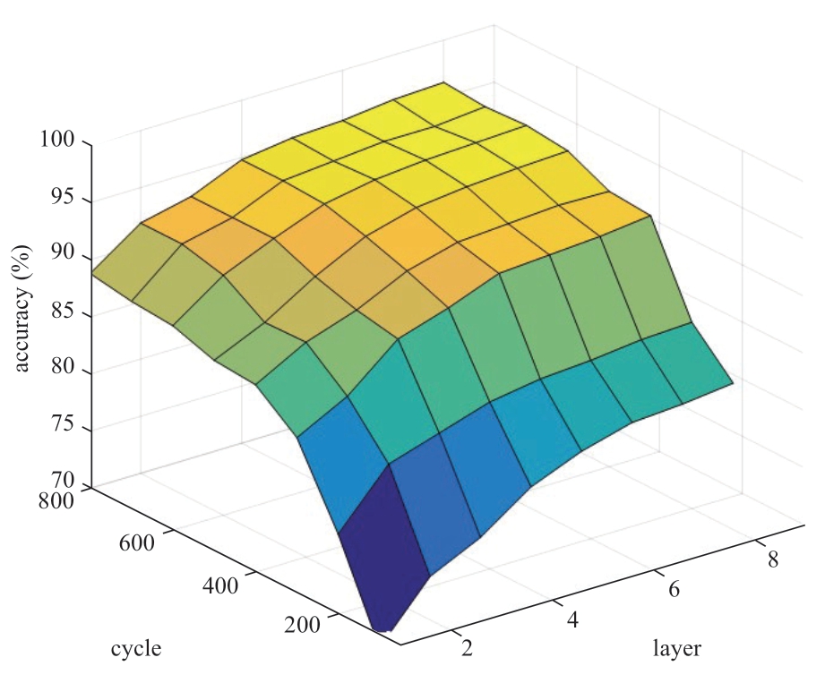
Fig.5 Relationships between the number of the network layers,the number of training cycles,and the identification accuracy rate

Ten characteristic parameters are inputted,resulting in nine fault causes.The network structure is 16–10–10–10–9.Based on this structure,the relationships between the selfdefined time(tk),wavelet decomposition level(n),and diagnostic accuracy rate can be found,as shown in Fig.6.Evidently,the effect of the diagnosis model is enhanced when tk and n are in the ranges 850–950 μs and 5–8,respectively.Accordingly,tk and n are modified and set to 900 μs and 6,respectively.

Based on the aforementioned network structure and parameters,the ADBN model is adopted for the fault diagnosis of the test samples.The derived confusion matrix is presented in Fig.7.As shown in Fig.6,the total recognition accuracy of the ADBN model can reach 94.6%.

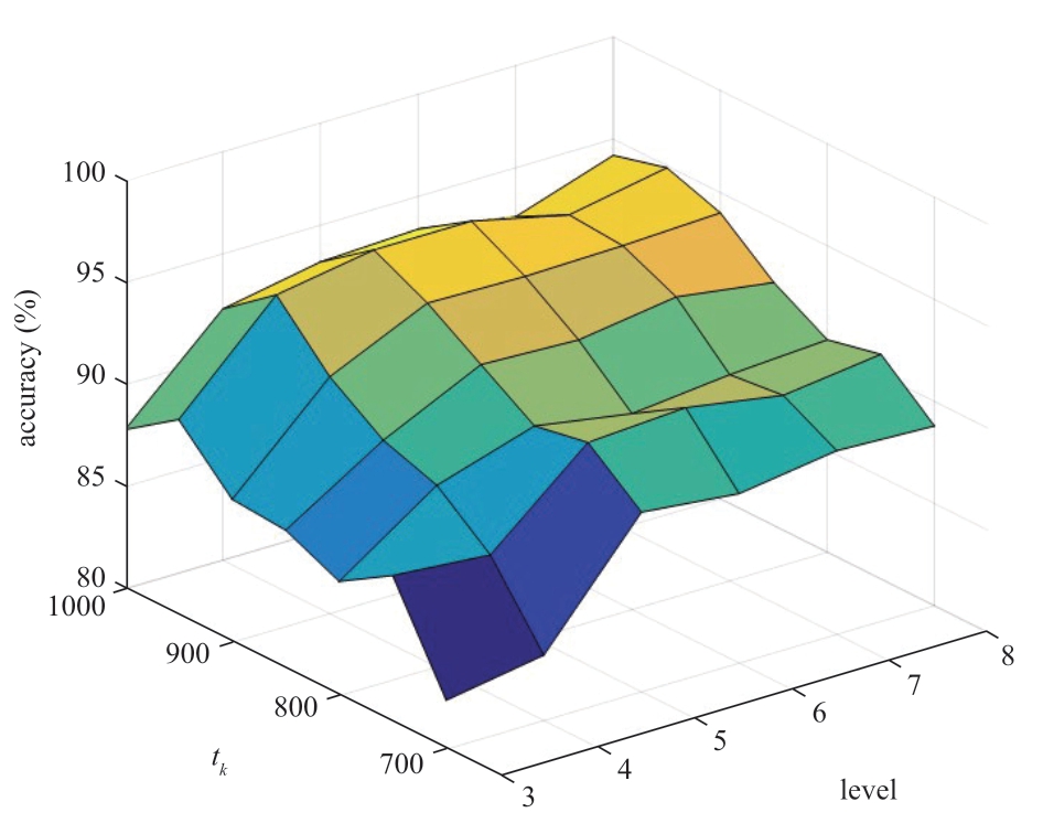
Fig.6 Relationships between the self-defined time tk,the wavelet decomposition level n,and the identification accuracy rate

Fig.7 Confusion matrix of recognition results

3.2 Comparison of different models and characteristic parameters

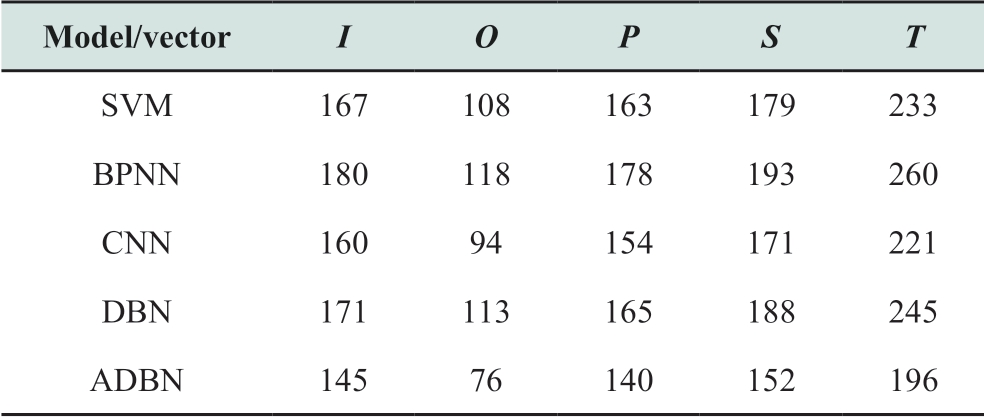
To evaluate the performance of the ADBN model,the fault causes are detected by adopting the SVM,backpropagation neural network(BPNN),convolutional neural network(CNN)[33],and DBN model.Among the feature parameters(T),T0 is the fault time period parameter;T1,T2,T3,T4,and T7 are the waveform time domain feature parameters; T5 and T6 are the waveform frequency domain feature parameters; and T8 and T9 are the new energy feature parameters.To confirm the rationality and applicability of T,different types of feature parameters are used as inputs to SVM,BPNN,CNN,and DBN.The feature parameters used for comparison are I=[T0,T1,T2,T3,T4,T7,T8,T9],which only includes time domain features; O=[T0,T5,T6,T8,T9],which only includes frequency domain features;P =[T0,T1,T2,T3,T6,T7,T8,T9],which includes some time–frequency features; and S=[T0,T1,T2,T3,T4,T5,T6,T7],which excludes new energy parameters.

Table 3 summarizes the fault diagnosis results of different models and characteristic vectors.Each recognition accuracy value listed in the table is the average of 15 calculation results.Evidently,the ADBN model exhibits higher recognition accuracy than the other models.The ADBN model with its vector,T,improves the fault diagnosis with a recognition accuracy rate exceeding 94%.

The recognition accuracy of the ADBN model compared with those of the SVM,BPNN,CNN,and DBN models,which apply T as the input feature parameter,increases by approximately 9%,11%,5%,and 3%,respectively.The accuracy of the ADBN model compared with that of the traditional DBN model has considerably improved.Additionally,when T is chosen as the input feature parameter,the model recognition accuracy significantly becomes better than that when other types of feature parameters are used.Consider the ADBN model as an example.Specifically,compared with using I,O,P,and S as feature parameters,when T is selected,the recognition accuracy rates improve by approximately 15%,24%,9%,and 8% respectively.The results indicate that the proposed characteristic parameter is reasonable and can completely depict the fault information included in diverse traveling waves.

The training times corresponding to different models and vectors are listed in Table 4.Vector T contains more fault information; consequently,model calculations are long and time consuming.When vector T is used as the input characteristic,the training times of the SVM,BPNN,CNN,DBN,and ADBN models are 233,260,221,245,and 196 s,respectively.Although the ADBN model structure is complex,it adopts the CD algorithm to perform layerby-layer pre-training and adaptively adjusts the learning rate according to each iteration direction of the parameters.Accordingly,the problems of under-learning and falling into local optimum can be avoided.Moreover,the speed of model convergence improved considerably.

Table 4 Training times(s)corresponding to different models and vectors

3.3 Influence of different sample sizes

To investigate the impact of sample size,the training samples are set to 500,800,2000,and 2800,and the number of testing samples is set to 200.With T as the characteristic vector,the resulting recognition accuracy is summarized in Table 5.Evidently,the accuracy rate of the ADBN model progressively increases with the number of samples.Moreover,the number of samples increases with the amount of characteristic information extracted from the ADBN model.Meanwhile,the internal relationship between electrical quantity and fault cause is more correctly identified.The transient electrical quantities in OTL faults vary with the line length,voltage level,fault location,new energy access ratio,and operating condition.The sample set is enlarged and enhanced depending on the OTL fault improvement,which contributes to the enhancement of the diagnostic effectiveness of the ADBN model.

Table 5 Recognition accuracy(%)corresponding to different sample sizes

3.4 Influence of new energy scale

In the simulation test step of the fault identification model,the influence of different proportions of wind turbines and photovoltaic power stations on the model is investigated.First,the wind turbine and photovoltaic power station are modeled using PSCAD/EMTDC,and the fault waveform corresponding to different faults is simulated.The scales of the wind turbine and photovoltaic power station are then adjusted to test the validity of the model.In addition,with full reference to the wind and solar resource divisions and subsequent development in different regions in China,wind and wind velocity ratio have been dynamically adjusted.For example,eastern China has numerous offshore wind power and distributed new energy,and western China has a number of centralized wind and solar bases.

In modeling the photovoltaic power station,the influence of solar incident angle and cloud shading factor on photovoltaic outputs is considered.The relationship between the characteristic parameters of meteorological conditions and photovoltaic output is studied.These parameters are transformed into the parameters in the probability model that affect the photovoltaic output.The conditional probability distribution of photovoltaic power generation,probability distribution function of photovoltaic output,attenuation coefficient of autocorrelation function,and matrix of spatial correlation coefficient are considered.

In terms of wind turbine modeling,the influence of total wind resources and wind speed uncertainty on wind power output is considered.A mathematical model of the influence of meteorological parameters on wind speed and wind volume in wind farms is established,and the conditional probability distribution of wind speed and total wind resources under different weather types are studied.The probability distribution function of wind power output,attenuation coefficient of autocorrelation function,and matrix of spatial correlation coefficient are considered.

We compared the scenarios of different new energy ratios based on the simulation test.The simulation results show that when the total installed capacity of wind turbines and photovoltaic power stations is in the range 5%–50%,the model recognition accuracy exceeds 92%.

In the test step of the fault identification model using actual data,3121 failure cases are classified.The grouping is based on the proportion of new energy sources connected to the overall power installation in the province(city)where the line fault occurs.The proportions of new energy access to the grid are classified as less than 10%,10%–20%,20%–30%,and greater than 30%.The numbers of fault cases in provinces(cities)where the proportions of new energy access to the grid are less than 10%,10%–20%,20%–30%,and more than 30% are 750,711,848,and 812,respectively.To examine the effect of the scale of new energy access to the grid on the model identification results,the number of fault cases corresponding to different new energy proportions must be consistent.To minimize the instability of fault identification due to small samples,the number of fault cases corresponding to different proportions of new energy sources must be increased to the maximum extent possible.Accordingly,the number of samples corresponding to the proportions of new energy sources is set to 711.

Different parameters are considered as input feature parameters,and the identification results of different models are summarized in Table 6.The results indicate that with T as the input parameter,in the case of different proportions of new energy access to the grid,the ADBN model identification accuracy rate is as high as 90%,and the variation range is less than 1%.The recognition effect is influenced to a certain extent if the input feature quantity does not include new energy parameters(considering parameter S as an example)or other models are used.As the proportion of new energy access to the grid increases,the effect of new energy parameters on the recognition accuracy also improves.

Table 6 Recognition accuracy(%)under different new energy scale scenarios

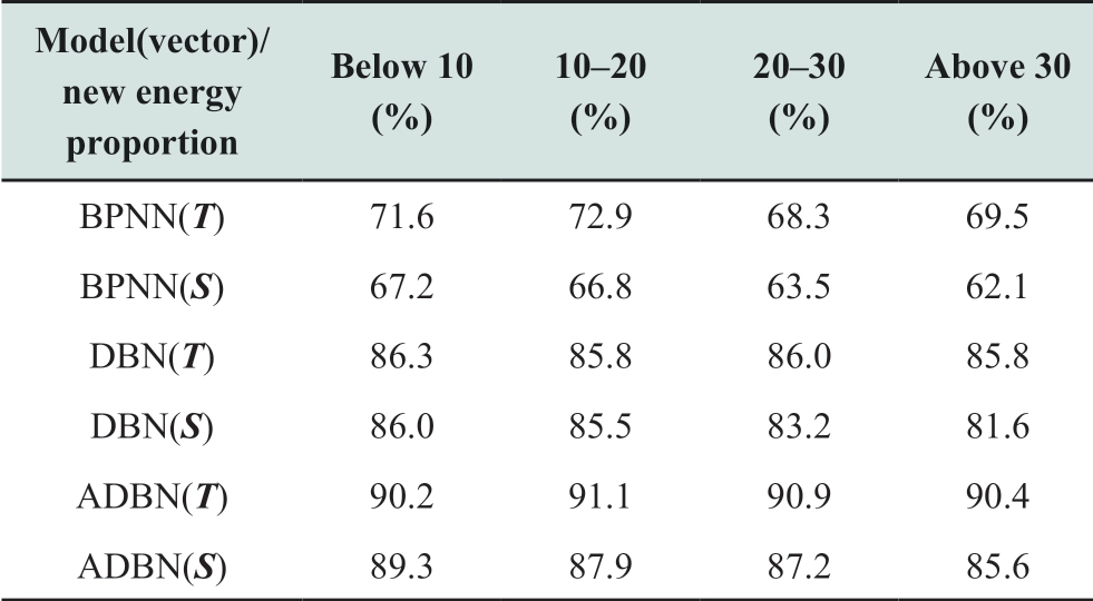
The results reveal that the new energy parameters selected in the study can completely reflect the scale of new energy access to the grid in the fault area.The model can effectively characterize the cause of the fault as well as the correlation between the fault waveform and new energy parameters.The method is applicable to different scales of new energy access scenarios.In the context of “carbon peak and carbon neutrality” objectives,the method remains applicable and effective.However,the increasing scale of new energy grid connection affects system characteristics.The increase in the number of failure cases also increases the fault samples corresponding to each new energy ratio and further improves the effect of method identification.

4 Conclusions

In the study,we investigated a transmission line fault identification method suitable for scenarios with high proportions of new energy access to the grid.Moreover,a model-driven and style="font-size: medium; text-align: justify; text-indent: 2em; line-height: 1.8em; margin: 0.5em 0em; color: rgb(0, 0, 0); font-family: SimSun; font-style: normal; font-variant: normal; font-weight: normal; letter-spacing: normal; orphans: auto; text-transform: none; white-space: normal; widows: 1; word-spacing: 0px; -webkit-text-stroke-width: 0px;">(1)The waveform characteristics of different fault types driving the model were investigated.Moreover,the time–frequency parameters in the fault waveform were fully explored.The parameters related to the moment of fault occurrence and new energy access to the grid as well as feature parameters related to fault causes were also identified.

(2)With respect to the style="font-size: medium; text-align: justify; text-indent: 2em; line-height: 1.8em; margin: 0.5em 0em; color: rgb(0, 0, 0); font-family: SimSun; font-style: normal; font-variant: normal; font-weight: normal; letter-spacing: normal; orphans: auto; text-transform: none; white-space: normal; widows: 1; word-spacing: 0px; -webkit-text-stroke-width: 0px;">(3)The study results suggest that the proposed model can efficiently identify nine fault causes under different scenarios.The overall recognition accuracy of the model considering different new energy access ratios was as high as 90%.

With the persistent increase in the proportion of gridconnected new energy sources,the expansion of fault cases may lead to changes in the classification of fault causes.The failure mechanism may also change to a certain extent.The occurrence of a certain fault may be due to a combination of various factors.

In the future,the mining method of fault characteristics can be further optimized.The internal correlation between different fault factors and fault causes can be studied in depth,and a more suitable fault identification model can be established.Moreover,the relationship between the actual fault data and evaluation results can be further explored.

Acknowledgements

This work was supported by State Grid Science and Technology Project(B3440821K003).

Declaration of Competing Interest

We declare that we have no conflict of interest.

References

[1] Xiong S H,Liu Y D,Fang J,et al.(2020)Incipient fault identification in power distribution systems via human-level concept learning.IEEE Transactions on Smart Grid,11(6):5239-5248

[2] Zheng T Q,Liu Y D,Yan Y J,et al.(2022)RSSPN:robust semisupervised prototypical network for fault root cause classification in power distribution systems.IEEE Transactions on Power Delivery,37(4):3282-3290

[3] Cong Z H,Liu Y D,Fang J,et al.(2020)Root-cause identification of single line-to-ground fault in urban small current grounding systems based on correlation dimension and average resistance.IEEE Transactions on Power Delivery,35(4):1834-1843

[4] Du Y,Liu Y,Shao Q,et al.(2020)Single line-to-ground faulted line detection of distribution systems with resonant grounding based on feature fusion framework.IEEE Transactions on power Delivery,34(4):1766-1775

[5] Li Z C,Liu Y D,Yan Y J,et al.(2021)An identification method for asymmetric faults with line breaks based on low-voltage side data in distribution networks.IEEE Transactions on Power Delivery,36(6):3629-3639

[6] Qin X,Liu Y D,Sun P,et al.(2017)Study on the line fault rootcause identification method in distribution networks based on time-frequency characteristics of fault wave-forms.Chinese Journal of Scientific Instrument,38(1):41-49(in Chinese)

[7] Wu H,Xiao X Y,Deng W J(2017)Identification of lightning strike and fault in the traveling wave location of transmission line.High Voltage Engineering,33(6):63-67(in Chinese)

[8] Wu T,Ruan J J,Zhang Y,et al.(2012)Study on the statistic characteristics and identification of AC transmission line trips induced by forest fires.Power System Protection and Control,2012,40(10):138-143+148(in Chinese)

[9] Núñez V B,Meléndez J,Kulkarni S,et al.(2013)Feature analysis and automatic classification of short-circuit faults resulting from external causes.International Transactions on Electrical Energy Systems,23(4):510-525

[10] Minnaar U J,Nicolls F,Gaunt C T(2016)Automating transmission-line fault root cause analysis.IEEE Transactions on Power Delivery,31(4):1692-1700

[11] Shu H C,Cao P L,Yang J J,et al.(2015)A method to distinguish between fault and lightning disturbance on transmis-sion lines based on CVT secondary voltage and CT secondary current.Transactions of China Electrotechnical Society,30(3):1-12(in Chinese)

[12] Malik H,Sharma R(2017)Transmission line fault classification using modified fuzzy Q learning.IET Generation,Transmission& Distribution,11(16):4041-4050

[13] Samantaray S R(2009)Decision tree-based fault zone identification and fault classification in flexible AC transmissionsbased transmission line.IET generation,transmission &distribution,3(5):425-436

[14] Jamehbozorg A,Shahrtash S M(2010)A decision-tree-based method for fault classification in single-circuit transmission lines.IEEE Transactions on Power Delivery,25(4):2190-2196

[15] Koley E,Shukla S K,Ghosh S,et al.(2017)Protection scheme for power transmission lines based on SVM and ANN considering the presence of non-linear loads.IET Generation,Transmission & Distribution,11(9):2333-2341

[16] Abdelgayed T S,Morsi W G,Sidhu T S(2018)Fault detection and classification based on co-training of semisupervised machine learning.IEEE Transactions on Industrial Electronics,65(2):1595-1605

[17] Silva K M,Souza B A,Brito N S D(2006)Fault detection and classification in transmission lines based on wavelet transform and ANN.IEEE Transactions on Power Delivery,21(4):2058-2063

[18] Yen J,Langari R(1999)Fuzzy logic:intelligence,control,and information.Upper Saddle River NJ:Prentice Hall

[19] Safavian S R,Landgrebe D(1991)A survey of decision tree classifier methodology.IEEE transactions on systems,man,and cybernetics,21(3):660-674

[20] Hssina B,Merbouha A,Ezzikouri H,et al.(2014)A comparative study of decision tree ID3 and C4.5.International Journal of Advanced Computer Science and Applications,4(2):13-19

[21] Hecht-Nielsen R(1992)Theory of the backpropagation neural network.Neural networks for perception.Pittsburgh:Academic Press,1992:65-93

[22] Schölkopf B,Smola A J,Bach F(2002)Learning with kernels,support vector machines,regularization,optimization,and beyond.Cambridge:MIT press

[23] Hinton G E(2009)Deep belief networks.Scholarpedia,4(5):5947

[24] Mohamed A,Dahl G,Hinton G(2009)Deep belief networks for phone recognition.Nips workshop on deep learning for speech recognition and related applications,Vancouver,Canada

[25] Le Roux N,Bengio Y(2008)Representational power of restricted Boltzmann machines and deep belief networks.Neural computation 20(6):1631-1649

[26] Lopes N,Ribeiro B(2014)Towards adaptive learning with improved convergence of deep belief networks on graphics processing units.Pattern Recognition,47(1):114-127

[27] Hinton G E(2002)Training products of experts by minimizing contrastive divergence.Neural computation,2002,14(8):1771-1800

[28] Carreira-Perpinan M A,Hinton G E(2005)On contrastive divergence learning.Aistats,Bridgetown,Barbados,10:33-40

[29] Sutskever I,Hinton G E,Taylor G W(2009)The recurrent temporal restricted boltzmann machine.Advances in neural infor-mation processing systems,Vancouver,British Columbia,Canada,1601-1608

[30] Salakhutdinov R,Hinton G(2009)Deep boltzmann machines.Artificial intelligence and statistics,Clearwater Beach,Florida,USA,448-455

[31] Liang H Q,Liu Y D,Sheng G H,et al.(2019)Fault-cause identification method based on adaptive deep belief network and time-frequency characteristics of travelling wave.IET Generation,Transmission & Distribution,13(5):724-732

[32] Unser M,Aldroubi A,Eden M(1992)On the asymptotic convergence of B-spline wavelets to Gabor functions.IEEE Transactions on Information Theory,38(2):864-872

[33] Chua L O,Yang L(1988)Cellular neural networks:Theory.IEEE Transactions on Circuits and Systems,35(10):1257-1272

Biographies

Hanqing Liang received Ph.D.degree at Shanghai Jiao Tong University in 2020.He is working in State Power Economic and Technological Research Institute Co.,Ltd.,Beijing,China.His research interests include fault diagnosis,renewable energy power generations,and power grid planning.

Xiaonan Han received M.S.degree at North China Electric Power University in 2012.She is working in State Power Economic and Technological Research Institute Co.,Ltd.,Beijing,China.Her research interests include power grid planning and grid economics.

Haoyang Yu received M.S.degree at London’s Global University in 2017.He is working in State Power Economic and Technological Research Institute Co.,Ltd.,Beijing,China.His research interests include renewable energy power generation and power grid planning.

Fan Li received Ph.D.degree at Tsinghua University in 2019.He is working in State Power Economic and Technological Research Institute Co.,Ltd.,Beijing,China.His research interests include power system reliability assessment,stability analysis and power grid planning.

Zhongjian Liu received Ph.D.degree at University of Bath in 2018.He is working in State Power Economic and Technological Research Institute Co.,Ltd.,Beijing,China.His research interests include power system stability analysis and power grid planning.

Kexin Zhang received M.S.degree at New York University in 2019.She is working in State Power Economic and Technological Research Institute Co.,Ltd.,Beijing,China.Her research interests include grid economics and renewable energy power generation.

(Editor Dawei Wang)